Verification of Numerical Technique for Hydraulic Fracturing Stimulation
- by Comparison with Analytical Solutions -
수압파쇄 설계를 위한 수치해석기법의 증명- 해석식과의 비교를 중심으로 -
Sim, Young-Jong† 심 영 종
ABSTRACT : Hydraulic fracturing technology has been widely applied in the industry for the recovery of the natural resources such as gas, oil and geothermal heat from hot dry rock. During hydraulic fracturing stimulation, multiple cracks are created resulting in mechanical interaction between cracks. Such an interaction influences obtaining hydraulic fracturing key parameters (crack opening, length, and borehole net pressure). The boundary collocation method (BCM) has been proved to be very effective in considering mechanical interaction. However, for better confidence, it needs to be verified by comparison with analytical solutions such as stress intensity factors. In this paper, three cases, single fracture in remote uniaxial tension, single fracture in remote shear stress field and two arbitrary segments in an infinite plane loaded at infinity are considered. As a result, the BCM is proved to be valid technique to consider mechanical interaction between cracks and can be used to estimate the hydraulic fracturing parameters such as opening of the fracture, and so on.
Keywords : Hydraulic fracturing, Boundary collocation method, Stress Intensity Factor
요 지 : 수압파쇄기술은 가스나 석유, 지열 등 자원추출을 하기 위해 다양한 분야에서 전세계적으로 응용되고 있는 기술이다. 이러 한 수압파쇄 작업 시 복수의 균열이 필수적으로 발생하여 균열간 기계적인 상호작용을 유발하는데 이러한 상호작용은 수압파쇄 시 얻어질 수 있는 결과(균열 폭, 균열 길이, 보어홀 내 압력)에 큰 영향을 끼치게 된다. 수치해석기법인 경계병치법은 이러한 균열 간의 역학적 상호작용을 고려하는데 유효한 수치해석적 기법으로 개발이 되고 있으나 응력확대계수를 계산하는 해석식과의 비교 등을 통한 검증이 필요하다. 이를 위해 무한평면에 일축 인장 응력과 전단응력이 작용하는 단일균열의 경우 및 임의의 두 균열이
존재하는 경우의 응력확대계수 및 균열폭 해석식과 본 수치해석기법을 통해 얻은 값을 비교하였다. 그 결과, 본 연구에서 제시한
경계병치법은 해석식과 상당히 근접한 결과를 나타내어, 균열간의 기계적인 상호작용을 고려하는데 유효함을 검증하였으며, 추후 수압파쇄 시 설계에 필요한 균열폭 등의 변수를 계산하는데 사용할 수 있음을 나타내었다.
주요어 : 수압파쇄, 경계병치법, 응력확대계수
† Member, Housing & Urban Research Institute, Senior Research Scientist(E-mail : [email protected]) 한국지반환경공학회 논문집
제10권 제4호 2009년 6월 pp. 65~71
1. Introduction
Hydraulic fracturing technology has been widely applied for the recovery of natural resources such as oil, gas, geo- thermal heat from hot dry rock (Fig. 1), waste disposal and remediation of contaminated water to create permeable reactive barrier (Fig. 2). During hydraulic fracturing stimulation, however, multiple fractures are expected to be created and mechanical interaction induced by fluid injection between fractures is essential. To consider mechanical interaction between fractures
(e.g., Naceur and Roegiers, 1990) is of great importance especially in the area of the recovery of natural resources because it affects fractures opening, length, and net pressure (difference between remote stress and internal pressure).
The boundary collocation method (BCM) is based on the primarily analytical derivations accounting for the mechanical interaction between fractures. This technique are, however, fairly complicated and, in many cases, not trivial. Sim et al.
(2006) and Sim and Kim (2005) have improved this tech- nique to visualize opening of the cracks induced by fluid
Fig. 1. Geothermal heat extraction (http://ww2.mne.ksu.edu/~geocrack/)
Fig. 2. Permeable reactive vertical barrier (Hocking, 2002)
q1(z1)
q2(z2) Δq1(z2)
Δq2(z1) p1 p2
x1 y1
x2 y2
= +
θ1
θ2
q1(z1)
q2(z2) Δq1(z2)
Δq2(z1) p1 p2
x1 y1
x2 y2
= +
θ1
θ2
Fig. 3. Principle of numerical technique for interacting with hydraulic fractures injection and have verified it by comparing opening with
that of finite element method. For better confidence in the version of the BCM developed in those papers, stress intensity factor (SIF) needs to be compared with other analytical solutions because SIF gives further information how crack will behave in the next. In this paper, therefore, SIF computed by the BCM are mainly compared with available analytical solutions.
2. Boundary Collocation Method (BCM)
The principle of the BCM has been introduced by Sim et al. (2006) by introducing a pair of interacting fractures in an infinite plane that are located at z1 and z2, respectively (Fig.
3). Known tractions, p1 and p2 are applied to the first and second fracture, respectively. Based on the superposition principle, this problem can be represented as a sum of two auxiliary problems for a single fracture. In the first auxiliary problem, unknown tractions acting on the first fracture q1
induce stresses Δq1 at the location of the second fracture.
Likewise, in the second auxiliary problem, unknown tractions loading the second fracture q2 generate stresses Δq2 at the location of the first fracture. Therefore, the tractions in the original problem can be written as
) ( ) ( ) ( ), ( ) ( )
( 1 2 1 1 1 2 2 1 2 2 2
1 z q z p z q z q z p z
q +Δ = +Δ = (1)
In this method, the complex potential is assumed to be an infinite series truncated to a finite number of collocation points.
These collocation points can be determined to satisfy prescribed boundary conditions. In this version of BCM, an approach using Chebyshev polynomials as an approximate function for the solution of multiple defects in an infinite homogeneous medium (e.g., Gladwell and England, 1977; McCartney and Gorley, 1987) are employed. As a result, stress intensity factors (SIF) and opening of the cracks, respectively, can be expressed as follows
( )
∑=
+ +
±
=
+ M
m
m m m II
I iK c i
K
1
) 1
1
( α β
π (2)
( )
∑= + −
−
= Δ +
Δ M
m
m m
m i U
m E
u c i v
1
1
2 1 ( )
' 1
4 ξ α β ξ
(3)
where KI is mode I SIF, KII is mode II SIF, c is the half size of the crack, m and m are real unknown coefficients to be determined, M is the number of collocation points, Um()
θ
∞
σyy
∞
σyy
θ
∞
σyy
∞
σyy
Fig. 4. Single inclined fracture in remote uniaxial tension
d considered fracture
remote fracture 2c
∞
σyy
∞
σyy
d considered fracture
remote fracture 2c
∞
σyy
∞
σyy
Fig. 5. Remotely spaced fracture (d = 100c)
Table 1. Comparison of computed SIFs with analytical solutions
KI KII
The BCM 0.5830 0.8330
Tada et al. (2000) 0.5831 0.8328
= sin((m+1)arcos())/sin(arcos()) is the mth order Chebyshev polynomial of the second kind, = x/c is the dimensionless coordinate along the crack, Δv is normal opening, Δu is shear opening, E′ = E/(1 - 2) for plane strain, E is the Young’s modulus, is the Poisson’s ratio, and + and - in (2) indicate SIFs for the case of > 0 and < 0, respectively.
3. Verification by Comparison with Avail- able Solutions
3.1 Single Fracture in Remote Uniaxial Tension A single inclined fracture in remote uniaxial tension is considered as shown in Fig. 4. The remote stress field is
given by xx∞
= 0, yy∞
= 1, and xy∞
= 0 while the fracture is inclined at an angle of = 55° with respect to the x-axis. Fracture half length is c = 1. Since the numerical code is developed for the case of more than two fractures (N ≥ 2), an auxiliary fracture can be placed at a distance of d = 100c such that their interaction becomes negligible as shown in Fig. 5. Therefore, both fractures can be considered as totally isolated from each other. Hereafter, the unit is not shown because it can be any type of unit system as long as it is used consistently in all parameters.
The analytical solution for SIF gives (Tada et al., 2000)
c KI σyy π θ π θ⎟ π
⎠
⎜ ⎞
⎝⎛ −
⎟⎠
⎜ ⎞
⎝⎛ −
= ∞
sin 2 sin 2
(4) c
KII σyy π θ π θ⎟ π
⎠
⎜ ⎞
⎝⎛ −
⎟⎠
⎜ ⎞
⎝⎛ −
= ∞
sin 2 cos 2
(5) The SIFs computed by the BCM show good agreement with analytical solutions (Table 1) showing 0.02% error for both KI and KII.
Normal and shear opening can be also calculated analy- tically based on (6) and (7) respectively. Poisson’s ratio
= 0.21 and Young’s modulus E = 1 are used as the elastic properties of the material. The analytical solutions for normal and shear opening (displacement discontinuities) are given by (Tada et al., 2000)
2 2 2
sin 2 sin 2
) 1 (
4 c x
v E y ⎟ −
⎠
⎜ ⎞
⎝⎛ −
⎟⎠
⎜ ⎞
⎝⎛ −
= −
Δ ν σ∞ π θ π θ
(6)
2 2 2
sin 2 cos 2
) 1 (
4 c x
u E y ⎟ −
⎠
⎜ ⎞
⎝⎛ −
⎟⎠
⎜ ⎞
⎝⎛ −
= −
Δ ν σ∞ π θ π θ
(7)
These normal and shear opening of the single inclined fracture (Fig. 4) are compared with the analytical solutions as shown in Fig. 6 and Fig. 7 and show good agreement.
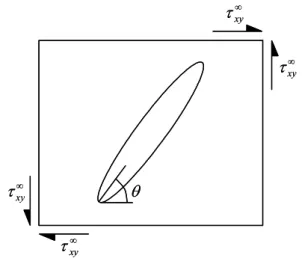
3.2 Single Fracture in Remote Shear Stress Field A single inclined fracture in a remote shear stress field is considered as shown in Fig. 8. The remote stress field is
1 0.8 0.6 0.4 0.2 0 0.2 0.4 0.6 0.8 1 0
0.5 1 1.5
Analytical solution The BCM
Distance along the fracture
Normal opening
Fig. 6. Comparison of normal opening with analytical solution
1 0.8 0.6 0.4 0.2 0 0.2 0.4 0.6 0.8 1
0 1 2
Analytical solution The BCM
Distance along the fracture
Shear opening
Fig. 7. Comparison of shear opening with analytical solution
θ
∞
τxy
∞
τxy
∞
τxy
∞
τxy
θ
∞
τxy
∞
τxy
∞
τxy
∞
τxy
Fig. 8. Single inclined fracture in remote shear stress field
Table 2. Comparisons of computed SIFs with analytical solution
KI KII
The BCM -1.6656 -0.6062
Tada et al. (2000) -1.6660 -0.6060
1 0.8 0.6 0.4 0.2 0 0.2 0.4 0.6 0.8 1
4 2 0
Analytical solution The BCM
Distance along the fracture
Normal opening
Fig. 9. Comparison of normal opening with analytical solution
1 0.8 0.6 0.4 0.2 0 0.2 0.4 0.6 0.8 1
1.5 1 0.5 0
Analytical solution The BCM
Distance along the fracture
Shear opening
Fig. 10. Comparison of shear opening with analytical solution
given by xx∞
= 0, yy∞
= 0, and xy∞
= 1 while the fracture is inclined at the same angle of = 55°. Fracture half length is c = 1. The auxiliary fracture is also placed at a distance of d = 100c such that their interaction become negligible.
An analytical solution for SIFs is (Tada et al., 2000)
c
KI =−τxy∞sin(2θ) π (8) c
KII =τxy∞cos(2θ) π (9)
Comparing with the analytical solutions in Table 2, the computed results by the BCM show 0.02% error for KI and 0.03% error for KII, in good agreement with the analytical solutions.
The analytical solutions for normal and shear openings are given by (Tada et al., 2000)
2 2 2
) 2 ) sin(
1 (
4 c x
v=− −E xy −
Δ ν τ∞ θ
(10)
2 2 2
) 2 ) cos(
1 (
4 c x
u= −E xy −
Δ ν τ∞ θ
(11) These normal and shear openings of the single inclined fracture (Fig. 8) are compared with analytical results as shown in Fig. 9 and Fig. 10 and show good agreement.
3.3 Two Arbitrary Segments in an Infinite Plane Loaded at Infinity
The asymptotic solution by Savruk and Datsyshin (1973) considers a fracture consisting of two equal, arbitrarily oriented segments in an infinite plane loaded at infinity. Stresses at infinity are xx∞
= 0.5, yy∞
= 1, and xy∞
= 0. The fracture configuration is summarized in Table 3 and plotted in Fig.
11. Two segments are located fairly far (d > c) from each other to make sure that the asymptotic solution is accurate.
The form of the solution presented by Savruk and Datsyshin (1973) depends upon two indices, n and k. One of them
Table 3. Configuration of two arbitrary segments that are located fairly far (d > c) from each other
Segment Center of segment (x, y)
Inclination angle
Half length c
1 (0, 0) -74° 1
2 (1, 5) 30° 1
Fig. 11. Two arbitrary segments in an infinite plane loaded at infinity
should be equal to one and the other, two. Therefore, the segment number is identified by a pair of digits (n, k). For example, (1, 2) represents the first segment while (2, 1) represents the second one. Savruk and Datsyshin’s (1973) solutions for KI on the left (KI_l) and right (KI_r) crack tips can be expressed as
⎟⎟
⎟⎟
⎟
⎠
⎞
⎜⎜
⎜⎜
⎜
⎝
⎛
⎟⎟ +
⎠
⎜⎜ ⎞
⎝
− ⎛ +
⎟⎟⎠
⎜⎜ ⎞
⎝ +⎛
− + +
=
+
∞
) , 256 ( ) , 32 ( ) 1 (
) , 16 ( ) 2 cos(
) 1 ( ) 1 ( 2
) 1 , (
3 4 2
3 1
1 2
_
k n I k n I
k n I c
k n K
k
n n
yy l
I λ λ
θ λ ε ε π σ
(12)
⎟⎟
⎟⎟
⎟
⎠
⎞
⎜⎜
⎜⎜
⎜
⎝
⎛
⎟⎟ +
⎠
⎜⎜ ⎞
⎝
− ⎛ +
⎟⎟⎠
⎜⎜ ⎞
⎝ +⎛
− + +
= ∞
) , 256 ( ) , 32 ( ) 1 (
) , 16 ( ) 2 cos(
) 1 ( ) 1 ( 2
) 1 , (
3 4 2
3
1 2
_
k n I k n I
k n I c
k n K
k
n n
yy r
I λ λ
θ λ ε ε π σ
(13)
where
( )
⎟⎟⎠
⎜⎜ ⎞
⎝
⎛
−
−
+
− +
−
−
− + +
−
−
−
− +
− +
=
)) 2 ( 2 cos(
2
)) (
2 cos(
)) (
2 cos(
) 2 cos(
)2 1 (
) 2
( 2 cos(
) ( 2 cos(
) ( 2 cos(
) 1 ( 2 ) ,
1(
n
k n n
k
n k n
k k
n I
θ β
θ θ β θ
θ β ε β
θ θ β θ
β β θ ε
(14)
⎟⎟⎠
⎜⎜ ⎞
⎝
⎛
−
− +
− +
−
− +
− − +
⎟⎟⎠
⎜⎜ ⎞
⎝
⎛
−
−
−
− +
− + +
=
) 3 5 cos(
3 ) 2 3 3 cos(
) 2 3 3 cos(
) 3 cos(
)3 1 (
) 3 2 5 cos(
3
)) ( 3 cos(
2 ) 3 2 cos(
)3 1 ( ) ,
2(
n k
n
k n n
n k
n n
k k
n I
θ β θ
θ β
θ θ β β ε θ
θ θ β
θ β β
θ ε θ
(15)
⎟⎟
⎟⎟
⎟⎟
⎟⎟
⎠
⎞
⎜⎜
⎜⎜
⎜⎜
⎜⎜
⎝
⎛
−
−
−
−
−
−
−
−
− +
−
+ +
−
−
+
− +
−
− +
−
−
−
− +
−
− +
−
− +
⎟⎟
⎟⎟
⎟
⎠
⎞
⎜⎜
⎜⎜
⎜
⎝
⎛
−
−
−
−
− +
+
−
−
−
− +
−
−
−
−
− +
− +
=
)) 2 ( 2 cos(
2 )) (
2 cos(
2
)) (
2 cos(
2 )) 2 ( 2 cos(
) 2 cos(
6
) 2 cos(
3 ) 2 cos(
10 )) 2 3 ( 2 cos(
24
)) 2 2 ( 2 cos(
6 )) 2 2 ( 2 cos(
7
)) 3
( 2 cos(
16 )) 2 ( 2 cos(
35
)) 2 2 ( 2 cos(
3 )) 2 ( 2 cos(
9
) 1 (
)) ( 2 cos(
2 )) ( 2 cos(
4
)) ( 2 cos(
2 5 )) 2 3 ( 2 cos(
14
)) ( 4 cos(
7 )) 2 3 ( 2 cos(
6
)) 2
( 2 cos(
20 )) ( 4 cos(
3 ) 1 ( 2 ) ,
3(
n k
n
n k n
k
k n
n
k n k
n
k n n
n k k
k k
n
k n k
n
n n
k
k n k
k n I
θ β θ
θ β
θ β θ θ
θ β
θ θ
θ β
θ θ β θ
θ β
θ θ β θ
β
θ θ β β
θ
ε
β θ θ
θ
θ θ θ
θ β
θ β θ
θ β
θ θ β β
θ ε
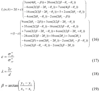
(16)
∞
∞
=
yy xx
σ ε σ
(17)
d c
=2
λ (18)
⎟⎟⎠
⎜⎜ ⎞
⎝
⎛
−
= −
1 2
1
arctan 2
x x
y β y
(19)
Their solutions for KII on the left (KII_l) and right (KII_r) crack tips can be expressed as
⎟⎟
⎟⎟
⎟
⎠
⎞
⎜⎜
⎜⎜
⎜
⎝
⎛
⎟⎟ −
⎠
⎜⎜ ⎞
⎝
− ⎛ +
⎟⎟⎠
⎜⎜ ⎞
⎝
−⎛
−
= ∞
) , 256 ( ) , 32 ( ) 1 (
) , 16 ( ) 2 sin(
) 1 ( 2
) 1 , (
3 4 2
3
1 2
_
k n II k n II
k n II c
k n K
k n n
yy l
II λ λ
θ λ ε π σ
(20)
⎟⎟
⎟⎟
⎟
⎠
⎞
⎜⎜
⎜⎜
⎜
⎝
⎛
⎟⎟ −
⎠
⎜⎜ ⎞
⎝
− ⎛ +
⎟⎟⎠
⎜⎜ ⎞
⎝
−⎛
−
=
+
∞
) , 256 ( ) , 32 ( ) 1 (
) , 16 ( ) 2 sin(
) 1 ( 2
) 1 , (
3 4 2
3 1
1 2
_
k n II k n II
k n II c
k n K
k n n
yy r
II λ λ
θ λ ε π σ
(21)
where
( )
⎟⎟⎠
⎜⎜ ⎞
⎝
⎛
−
−
+
− +
−
− − +
−
−
−
− +
=
)) 2 ( 2 sin(
2
)) (
2 sin(
) (
2 )sin 1 (
)) 2
( 2 sin(
)) ( 2 sin(
) 1 ( 2 ) ,
1(
n
k n n
k
n k
k n
n II
θ β
θ θ β θ
θ ε β
θ θ β θ
β ε
(22)
⎟⎟⎠
⎜⎜ ⎞
⎝
⎛
−
− +
− +
−
− +
− − +
⎟⎟⎠
⎜⎜ ⎞
⎝
⎛
−
−
−
− +
− + −
=
) 3 5 sin(
3 ) 2 3 3 sin(
) 2 3 3 sin(
) 3 ) sin(
1 (
) 3 2 5 sin(
3
)) ( 3 sin(
2 ) 2 3 )sin(
1 ( ) ,
2(
n k
n
k n n
n k
n n
k k
n II
θ β θ
θ β
θ θ β θ ε β
θ θ β
θ β θ
θ ε β
(23)
⎟⎟
⎟⎟
⎟⎟
⎟⎟
⎠
⎞
⎜⎜
⎜⎜
⎜⎜
⎜⎜
⎝
⎛
−
−
−
−
−
−
−
−
− +
−
+
−
−
−
+
− +
−
− +
−
−
−
− +
−
− +
−
− +
⎟⎟
⎟
⎠
⎞
⎜⎜
⎜
⎝
⎛
−
−
− +
−
−
−
− +
−
−
−
−
− +
=
)) 2 ( 2 sin(
2 )) (
2 sin(
2
) (
2 sin(
2 )) 2 ( 2 sin(
) 2 sin(
2
) 2 sin(
) 2 sin(
6 )) 2 3 ( 2 sin(
24
)) 2 2 ( 2 sin(
6 )) 2 2 ( 2 sin(
7
)) 3
( 2 sin(
16 )) 2 ( 2 sin(
23
)) 2 2 ( 2 sin(
3 )) 2 ( 2 sin(
) 1 (
)) ( 2 sin(
4 )) ( 2 sin(
2
)) 2 3 ( 2 sin(
28 )) ( 4 sin(
14
)) 2 3 ( 2 sin(
12 )) 2
( 2 sin(
26 ) 1 ( ) ,
3(
n k
n
n k n
k
k n n
k n k
n
n k n
n k k
n n
k
k n n
n k k
n
k n II
θ β θ
θ β
θ β θ θ
θ β
θ θ θ
β
θ θ β θ
θ β
θ θ β θ
β
θ θ β θ
β ε
θ β θ
θ
θ θ β θ
β
θ θ β θ
θ β ε
(24)
As shown in Table 4 and 5, the computed results are close to those of the asymptotic solutions by Savruk and Datsyshin (1973). These results are also compared with those calculated by Galybin’s (Astakhov et al., 2000) code, which numerically
Table 4. Comparisons of KI with asymptotic solutions by Savruk and Datsyshin (1973)
Segment Asymptotic solution The BCM
Left Right Left Right
1 KI_l = 0.966 KI_r = 0.983 KI_l = 0.967 KI_r = 0.983 2 KI_l = 1.557 KI_r = 1.559 KI_l = 1.555 KI_r = 1.557
Table 5. Comparisons of KII with asymptotic solutions by Savruk and Datsyshin (1973)
Segment Asymptotic solution The BCM
Left Right Left Right
1 KII_l = -0.221 KII_r = -0.230 KII_l = -0.222 KII_r = -0.229
2 KII_l = 0.419 KII_r = 0.405 KII_l = 0.419 KII_r = 0.405
Table 6. Stress intensity factors calculated by Galybin’s code
Segment KI KII
Left Right Left Right
1 KI_l = 0.967 KI_r = 0.983 KII_l = -0.222 KII_r = -0.229 2 KI_l = 1.555 KI_r = 1.557 KII_l = 0.419 KII_r = 0.405
Table 7. Configuration of two arbitrary segments that are located closely
Segment Center of segment (x, y)
Inclination angle
Half length c
1 (1, 0.9) 40° 1.2
2 (0.9, 2.1) -30° 0.7
Fig. 12. Two arbitrary segments in an infinite plane loaded by internal pressure
Table 8. Comparisons of KIwith the results by Galybin’s (Astakhov et al., 2000) code
Segment Galybin’s code The BCM
Left Right Left Right
1 KI_l = 3.863 KI_r = 4.128 KI_l = 3.862 KI_r = 4.123 2 KI_l = 1.426 KI_r = 2.996 KI_l = 1.427 KI_r = 2.997
Table 9. Comparisons of KII with the results by Galybin’s (Astakhov et al., 2000) code
Segment Galybin’s code The BCM
Left Right Left Right
1 KII_l = -6.075 KII_r = -6.154 KII_l = -6.075 KII_r = -6.155 2 KII_l = 2.422 KII_r = 3.203 KII_l = 2.422 KII_r = 3.203
calculates SIFs for the same fracture configuration. SIFs by Galybin’s (Astakhov et al., 2000) code are very similar to those obtained by the BCM and the asymptotic solutions
(Savruk and Datsyshin, 1973) as shown in Table 6.
Although BCM results for SIFs match the asymptotic solution and Galybin’s (Astakhov et al., 2000) code results closely enough, the difference between SIFs on different segment ends is not too large because the segments are located fairly far from each other. To have an independent comparison, the BCM is tested against Galybin’s (Astakhov et al., 2000) code for a configuration (Table 7 and Fig. 12) of non-equal segments loaded by different internal pressure and with more significantly varying SIFs on both ends. The internal pressure for two segments are p1 = 2 and p2 = 1 respectively. As a result, the agreement between the two sets of results for SIFs obtained by independent codes is nearly ideal as shown in Table 8 and Table 9.
4. Conclusions
The boundary collocation method is verified by comparison of computed SIFs and openings with those of analytical solutions. Three cases, single fracture in remote uniaxial tension, single fracture in remote shear stress field and two arbitrary segments in an infinite plane loaded at infinity are considered. As a result, the SIFs and opening of the cracks are good agreement with analytical solutions. Therefore, the BCM can be extensively applied to estimate hydraulic fracturing parameters such as opening of the fracture where the mechanical interaction between fractures is expected.
References
1. Astakhov, D.K., Sim, Y.J. and Germanovich, L.N. (2000),
MultiFrac2000, User Manual, Georgia Institute of Technology, p 235.
2. Gladwell, G.M.L. and England, A.H. (1977), Orthogonal Polynomial Solutions to Some Mixed Boundary-Value Problems in Elasticity Theory, Quarterly Journal of Mechanics and Applied Mathematics, Vol. 30, pp. 175~185.
3. Hocking, G. and Wells, S. (2002), Design, Construction and Installation Verification of a 1200 Long Iron Permeable Reactive Barrier, 8th Annual Florida Remediation Conference, p. 9.
4. McCartney, L.N. and Gorley, T.A.E. (1987), Complex Variable Method of Calculating Stress Intensity Factors for Cracks in Plates, Numerical Methods in Fracture Mechanics, Proceeding of the 4th International Conference, San Antonio, pp. 55~72.
5. Naceur, K.B. and Roegiers, J.-C. (1990), Design of Fracturing Treatments in Multilayered Formations, SPE Production Engi- neering, pp. 21~26.
6. Savruk, M.P. and Datsyshin, A.P. (1973), On the Limiting State of Equilibrium of a Plate Weakened by Two Arbitrarily- Oriented Cracks, Physico-Mechanical Institute, Academy of Sciences of the Ukrainian SSR, L’vov. Translated from Prikladnaya Mechanika, Vol. 9, No. 7, pp. 49~56.
7. Sim, Y.J. and Kim, H.T. (2005), A Study on the Interaction of Segmented Hydraulic Fractures, Journal of the Korean Geotechnical Society, Vol. 21, No. 9, pp. 45~52.
8. Sim, Y.J., Kim, H.T. and Germanovich, L.N. (2006), Study on the Fracture Deformation Characteristics in Rock by Hydraulic Fracturing, Journal of the Korean Geo-Environmental Society, Vol. 7, No. 2, pp. 43~53.
9. Tada, H., Paris, P.C. and Irwin, G.R. (2000), The Stress Analysis of Cracks Handbook, American Society of Mechanical Engineers, 3rd Ed., p. 696.
(접수일: 2009. 4. 16 심사일: 2009. 4. 28 심사완료일: 2009. 5. 12)