韓 國 水 資 源 學 會 論 文 集 第44卷 第6號 2011年 6月
pp. 429~438
< ISE 수자원학회 특별호 논문 >
Free Surface Flow in a Trench Channel Using 3-D Finite Volume Method
Lee, Kil Seong* / Park, Kidoo** / Oh, Jin-Ho***
...
Abstract
In order to simulate a free surface flow in a trench channel, a three-dimensional incompressible unsteady Reynolds-averaged Navier-Stokes (RANS) equations are closed with the model. The artificial com- pressibility (AC) method is used. Because the pressure fields can be coupled directly with the velocity fields, the incompressible Navier-Stokes (INS) equations can be solved for the unknown variables such as velocity components and pressure. The governing equations are discretized in a conservation form using a second order accurate finite volume method on non-staggered grids. In order to prevent the oscillatory behavior of computed solutions known as odd-even decoupling, an artificial dissipation using the flux- difference splitting upwind scheme is applied. To enhance the efficiency and robustness of the numerical algorithm, the implicit method of the Beam and Warming method is employed. The treatment of the free surface, so-called interface-tracking method, is proposed using the free surface evolution equation and the kinematic free surface boundary conditions at the free surface instead of the dynamic free surface boundary condition. AC method in this paper can be applied only to the hydrodynamic pressure using the decomposition into hydrostatic pressure and hydrodynamic pressure components. In this study, the boundary-fitted grids are used and advanced each time the free surface moved. The accuracy of our RANS solver is compared with the laboratory experimental and numerical data for a fully turbulent shallow-water trench flow. The algorithm yields practically identical velocity profiles that are in good overall agreement with the laboratory experimental measurement for the turbulent flow.
Keywords: free surface flow, unsteady Reynolds-averaged Navier-Stokes (RANS) equations, model, artificial compressibility (AC) method, finite volume method, interface-tracking method, hydro- dynamic pressure
...
* Professor, Department of Civil and Environmental Engineering, Seoul National University, 599 Gwanak-ro, Gwanak-gu, Seoul 151-744, Korea
**Corresponding Author, Ph.D., Candidate, Department of Civil and Environmental Engineering, Seoul National University, 599 Gwanak-ro, Gwanak-gu, Seoul 151-744, Korea. Tel: 82-2-880-8345, Fax: 82-2-873-2684, E-mail: [email protected]
*** Master. Student, Department of Civil and Environmental Engineering, Seoul National University, 599 Gwanak-ro, Gwanak-gu, Seoul 151-744, Korea
DOI: 10.3741/JKWRA.2011.44.6.429
1. INTRODUCTION
The two-dimensional vertically averaged shallow water equations have been commonly applied to the most of the hydraulic engineering flows during the last
two decades. Three-dimensional (3D) numerical models are required to compute the vertical and transverse variation of velocity at the natural river, the compli- cated channels, and estuarial regions. 3D free-surface models based on the hydrostatic pressure for free-
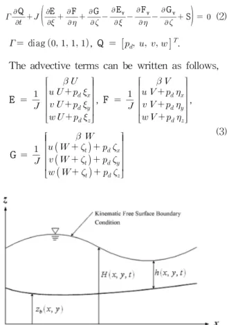
Fig. 1. Definition of the Water Surface and the Bottom Elevation
surface flow approximation have been developed lately.
The hydrostatic models (Casulli and Cheng, 1992;
Huang and Spaulding, 1995; Lu and Wai, 1998) assumed that the vertical acceleration components are very small.
However, when the depth is small to be compared with the wave length, its assumption is not available for the abruptly changing bed topography, short wave motion, and the problem of the saltwater intrusion with strong density gradients. In recent years, the hydrodynamic models have been developed beyond limitations of the hydrostatic pressure assumption (Casulli and Stelling, 1998; Casulli, 1999; Stelling, 2001; Musteyde et al., 2002;
Yuan and Wu, 2004; Lee et al., 2006a). A fractional step method, that the pressure is decomposed into the hydrostatic and the hydrodynamic pressure components, has been employed by Casulli and Stelling, Casulli, Stelling, Musteyde et al., Yuan and Wu, and Mahadevan et al.. Because the hydrodynamic pressure component as a function of the velocity field in a fractional step method is unknown, an integrated time step using two fractional steps is employed for a fractional step method. The first step is that velocity components in momentum equations are solved with hydrodynamic pressure components at previous time step. It introduces the errors of mass conservation in the incompressible continuity equation.
Corrected velocities, which can be computed to solve the pressure-Poisson equation at the second step, can be eliminated to determine the hydrodynamic pressure.
The CPU time is very expensive to solve the pressure- Possion equation using a fractional step method.
The artificial compressibility (AC) method instead of a fractional step method was originally proposed by Chorin (1967) for solving the steady state incompres- sible Navier-Stokes equations through a time-marching approach. It is called well established time-marching methods. According to this formulation the continuity equation is transformed from a constraint imposed on the velocity field to an evolution equation in time, by adding a time derivative of the pressure to it. The AC method, directly coupled with pressure and velocity field, was developed by Beddhu et al. (1994), Li (2003), and Lee et al. (2006).
In this paper, we present the three dimensional in- compressible unsteady Reynolds-averaged Navier- Stokes (RANS) equations closed with unsteady stati-
stical turbulence model, which is incorporated into the standard model. AC method is employed only to the hydrodynamic pressure using the decomposition into hydrostatic and hydrodynamic components (Lee et al., 2006b).
2. MATHEMATICAL FORMULATION For free surface flows (Lee et al., 2006b), the pressure term can be decomposed into two components such as the hydrostatic pressure and the hydrodynamic pressure (Fig. 1), leading to,
(1) where is the function of the vertical locationand water surface elevation , and . is a water density, and is a gravitational acceleration.
2.1 Governing Equations
Using the generalized curvilinear coordinate trans- formations, the Navier-Stokes equations can be for- mulated in vector form as follows,
Q
E
F
G
Ev
Fv
Gv
S (2)
diag , Q .
The advective terms can be written as follows,
E
, F
,
G
(3)
where is the artificial compressibility parameter., , and are velocity components. is the time, and the relationship between contravariant velocity components and covariant velocity components is as follows,
(4)
where the derivatives are called the metrics. The Jacobian of the geometric transformation → is defined as follows,
(5) The diffusion terms can be also written as follows,
Ev
Fv
Gv
where is the so-called contravariant metric tensor and is the velocity gradient tensor.
The gravity terms can be also written as follows,
S
(7)2.2 Standard Model
The standard model is employed in order to compute the eddy viscosity as to close the RANS equations. In the standard model, the eddy viscosity is calculated in terms of the turbulence kinetic
energy and its rate of dissipation . The transport equations for and are formulated in curvilinear coordinates using the vector form as follows,
Qt
Et
Ft
Gt
Ev
t
Fv
t
Gv
t St (8)
where Qt (9)
Et
, Ft
, Gt
(10)
Ev
t
Fv
t
(11)Gv
t
St
(12)
This model contains five parameters and the most commonly used values are as follows,
. (13) The rate of production of turbulent kinetic energy by mean flow represents to transfer kinetic energy from the mean flow to the turbulence. Because the eddy viscosity hypothesis is used, the rate of production of turbulent kinetic energy can be written,
. (14)The eddy viscosity is expressed as,
. (15)
(6)
3. NUMERICAL METHODS
The unsteady Reynolds averaged Navier-Stokes (RANS) equations in generalized curvilinear coordinates with the mean flows and turbulence closure equations are marched by integrating a time using the discrete equations.
3.1 Discretization for RANS Equations and Turbulence Transport Equations
The RANS equations are discretized in the conser- vation form using a three-point backward, second- order accurate Euler implicit scheme for the temporal derivative and three-point, second order accurate central differencing for the spatial derivatives,
(16)
where diag
∆
, (17)
∆
. (18)
The flux is the flux at the cell interfaces and the artificial dissipation flux is chosen as the matrix- valued scheme (Lin and Sotiropoulos, 1997),
(19)
(20) where is a constant and the Jacobian matrix is . The turbulence transport equations are discretized in space and time. The numerical scheme of the turbul- ence transport is a similar to that of the RANS equations as follows,
. (21)
The governing equations are discretized in a con- servation form using a second order accurate finite volume method on a non-staggered grid. To enhance the efficiency and robustness of the algorithm, the local dual time stepping and the implicit method of the
Beam and Warming method, which is the extension of the ADI method (Beam and Warming, 1967), are employed.
3.2 Boundary Conditions
Boundary conditions are specified at the inlet, outlet, and solid wall boundaries. Boundary conditions are needed for the model equations. In this section, the boundary conditions for equations in the open channel hydraulics are described in detail. The numerical scheme for advancing and is unchanged from the scheme with the hydrostatic pressure assumption using the standard bed and the surface boundary conditions.
At the inlet, the velocity components and turbulence variables are specified for open channel flow (Chow, 1959)
ln
Rough bed
ln
Smooth bed
(22)
where is equivalent roughness height, and is the friction velocity, is called the von Karman constant, is kinematic viscosity, is the turbulence model parameter, and is the flow depth. If inlet boundary conditions in Eq. (22) are simplified, its boundary conditions for the homogeneous turbulence can be specified as,
constant
(23)
At the outlet, is defined and zero normal gradients are specified for all the other variables.
At the free surface, and are defined (Rodi, 1984) by
(24)
where is the coordinate normal to free surface.
At the free surface and a zero normal gradient condition for andare used. The vertical velocity at the free surface is determined from the kinematic boundary condition,
. (25)
3.3 Free Surface Evolution Equation
As shown in Fig. 1, the original incompressible continuity equation is integrated over the depth in order to get the water surface equation. Using the generalized curvilinear coordinate transformations, the free surface equation can be derived (Lee et al., 2006a and 2006b),
(26)
whereis the depth,is the bottom elevation, and the transformed velocities are as follows,
(27)
3.4 Wall Boundary Conditions Using Wall Func- tions
The inner part of the wall layer, right next to the wall, is dominated by viscous effects and it is called the viscous sublayer. In spite of the fluctuations, the Reynolds stresses are still small here because of the viscous effects. Because of the thinness of the viscous sublayer, the stress can be taken as uniform within the layer and equal to the wall shear stress . The velocity distribution of Eq. (28) is linear and no-slip boundary condition is available in the viscous sublayer,
at ≤ . (28) The inner and outer solutions are matched together in a region of overlap. These velocity distributions are in the overlap layer, called the inertial sublayer or simply the logarithmic layer,
ln
for rough walls at
(29)
ln
ln
for smooth walls at
(30)
where is the velocity parallel to boundary which is calculated from the momentum equations at , the nor- mal distance of the first grid point from the boundary,
is nondimensional velocity, is the friction velocity which is related to the bottom shear stress, and is the roughness height. The wall func- tion is valid when ms at ≤ ≤ , and the grid allocation varies from m to
m (Stansby and Zhou, 1998; Lee et al., 2006b).
Because no-slip boundary condition at the wall is not used to reduce the grid size, the wall function is applied in this study.
3.5 Vertical Grid Generation
Horizontal grids are generated depending on the geometrical boundaries. However, along the vertical direction, when inviscid flow of constant eddy viscosity is assumed, the water depth is divided using an equally spaced vertical grid. For the turbulent flows, since the spacing of vertical grid near the bottom is finer than that of center for vertical direction, the following alge- braic equations using a grid clustering method may be employed by Hoffmann & Chiang (2000). The inverse transformation is given by
(31)
where is the clustering parameter, and defines where the clustering takes place.
3.6 Solution Procedure for Free Surface Treat- ment
A more accurate treatment of the free surface is proposed in this study which uses the free surface equation and kinematic boundary condition. At the
(b) Computational Domain Along the Center Line at m (a) 3-D Computational Domain for the Trench Channel Fig. 2. Flow Chart of 3-D Numerical Solver
beginning of the computation, the free surface is assumed flat and a mesh is generated. During the iterative solution process, the kinematic boundary condition is enforced through the vertical velocity boundary condition while the free surface equation is
used to obtain the free surface elevation. When the new surface elevation is obtained, the grid is generated through stretch or compression to conform to the new free surface shape. The flow chart of 3-D numerical solver, which is developed in this study, is shown in Fig. 2. This numerical solver consists of two time iteration loops (such as a real time step iteration loop and a pseudo-time step iteration loop), the module of a free-surface evolution, and finally, the module of a grid generation for a free surface.
3.7 Application Case
The experiment of van Rijn (1982) who measured the velocities, turbulent kinetic energy, shear stress for the trench channel is selected as a test case in this paper. In this trench channel flow, numerical solutions with the model are compared with experimental results in a channel m long and m wide with
m high side walls (Alfrink and van Rijn, 1983;
Stansby and Zhou, 1998; Basara and Younis, 1995;
Lee et al., 2006b). The computational domain initially consists of an equally spaced grid m used in the
Fig. 4. Velocity Profiles for the Trench Channel Flow Along the Center Line
Fig. 5. Turbulent Kinetic Energy Profiles for the Trench Channel Flow Along the Center Line
Fig. 6. Shear Stress Profiles for the Trench Channel Flow Along the Center Line horizontal and lateral directions with 31 layers in the
vertical direction using and in Eq. (31).
In order to evaluate the performance of this numerical method, mesh sizes are chosen: the finest mesh is 225
× 11 × 31 nodes. A coarser mesh is 113 × 11 × 31 nodes.
And the coarsest mesh is 57 × 11 × 31 nodes. The most optimal and convenient value of to get the most acceptable convergence is selected to the unity through several computational experiments performed by some authors (Roger and Kwak, 1991; Kaliakatsos et al., 1996; Chen et al., 1999; Madsen and Schaffer, 2006). The Courant-Friedrich-Lewis () number used in this numerical study is . As shown
in Fig. 3, five measurement locations at m,
m, m, m and m along the longitudinal direction are where observed data are compared with numerical results in this study.
4. RESULTS
As shown from Fig. 4 to Fig. 6, this algorithm yields good agreement with van Rijn’s experimental results for the horizontal velocity , turbulent kinetic energy
, and shear stress. The model predicts the largest discrepancy near the bottom at locations m and m. At these locations, the results of finer
Fig. 7. Velocities at Location m According to Grid Sizes
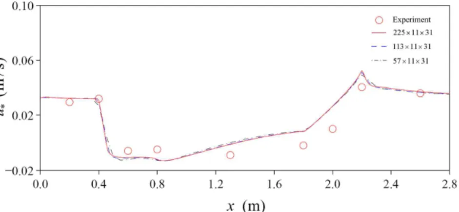
Fig. 9. Friction Velocities, According to Grid Resolution
Fig. 8. Velocities at Location m According to Grid Sizes
grids show more accuracy than those of the coarser grid near the bottom. The difference of shear stress profiles between experimental and numerical results is larger along direction. This is because that a model is assumed for an isotropic turbulence.
Especially, in order to examine grid dependency, numerical solutions are obtained using three computa- tional domains, which are refined in the longitudinal direction such as 57 × 11 × 31 nodes, 113 × 11 × 31 nodes, and 225 × 11 × 31 nodes. The vertical grid spacing is computed using and in Eq. (31).
Because the vertical grid size is sufficient enough to solve the wall boundary, only longitudinal direction is refined in this study. From Fig. 7 to Fig. 8, the longitu- dinal velocities according to each grid size are com- pared at locations m and m, where reversal flow is observed and where velocities vary rapidly compared to the other locations.
As shown in Fig. 9, the friction velocities are com- puted with these different grids, and the results for the friction velocities are compared, where relatively large differences are shown depending on the different grids for the hydrodynamic pressure calculations near the beginning and the end of the trench. Fig. 9 shows that larger grid sizes should be required if accurate estimation of shear velocities is important.
However, the numerical solutions calculated from this model are as good as the experimental data by van Rijn (1982). This indirectly means more accuracy and applicability of the current AC method by solving hydrodynamic pressure and velocities simultaneously.
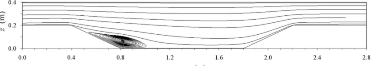
Streamlines show that a circulation pattern occurs near the beginning of the trench in Fig. 10 and the same circulation pattern for velocity vectors is also shown in Fig. 11.
Fig. 10. Streamlines of Computation with Hydrodynamic Pressure Along the Center Line
Fig. 11. Velocity Profiles of Computation with Hydrodynamic Pressure Along the Center Line
5. CONCLUSION
We have developed numerical scheme for incor- porating the hydrodynamic pressure using the artificial compressibility method at trench channel problem. The numerical model is formulated in gener- alized curvilinear coordinates in conservation form and model is incorporated for the turbulence closure. In this numerical method, the advection terms are approximated using the second order accurate central differencing with the artificial dissipation flux chosen as the matrix-valued scheme. In this study, the trench flow problem for the steady state test case is applied because experimental data are available.
Reasonable agreement with experimental results is found in this trench problem.
ACKNOWLEDGEMENT
This research was supported by the Social Infra- structure Research Group for Safe and Sustainable Development of the BK21 program (80%), and the Integrated Research Institute of Construction and Environmental Engineering (20%). This work was conducted at the Engineering Research Institute of Seoul National University, Seoul, Korea. The second author is grateful to Dr. Jong Wook Lee at Murray- Darling Basin Authority, Australia for his advice developing the numerical method in this study.
REFERENCES
Alfrink, B.J., and van Rijn, L.C. (1983). Two-equation turbulence model for flow in trenches. Journal of Hydrologic Engineering, Vol. 109, pp. 941-958.
Basara, B., and Younis, B.A. (1995). Prediction of tur- bulent flows in dredged trenches.Journal of Hydraulic Research, Vol. 33, pp. 813-824.
Beam, R.M., and Warming, R.F. (1978). An implicit finite-difference algorithm for hyperbolic systems in conservation-law form. Journal of Computational Physics, Vol. 22, pp. 87-110.
Beddhu, M., and Tayloe, L.K. (1994). A time accurate calculation procedure for flow with a free surface using a modified artificial compressibility formula- tion. Applied Mathematics and Computation, Vol.
65, pp. 33-48.
Casulli, V. (1999). A semi-implicit finite difference method for non-hydrostatic, free-surface flows.Inter- national Journal for Numerical Methods in Fluids, Vol. 30, pp. 425-440.
Casulli, V., and Busnelli, M.M. (2001). Numerical simu- lation of the vertical structure of discontinuous flow.
International Journal for Numerical Methods in Fluids, Vol. 37, pp. 23-43.
Casulli, V., and Cheng, R.T. (1992). Semi-implicit finite difference methods for three-dimensional shallow water flow. International Journal for Numerical Methods in Fluids, Vol. 15, pp. 629-648.
Casulli, V., and Stelling, G.S. (1998). Numerical simula- tion of three dimensional, quasi-hydrostatic free- surface flows. Journal of Hydraulic Engineering, ASCE, Vol. 124, No. 7, pp. 678-686.
Chorin, A. (1967). Numerical solution of Navier-Stokes equations for an incompressible fluid.Bulletin of the American Mathematical Society, Vol. 73, No. 6, pp.
928-945.
Chow, V.T. (1956).Open-channel Hydraulics. New York, McGraw-Hill.
Ferziger, J.H., and Peric, M. (1996). Computational Methods for Fluid Dynamics, Springer-Verlag, Berlin Heidelberg.
Hoffmann, K.A., and Chiang, S.T. (1993). Computa- tional Fluid Dynamics for Engineers, Engineering Education System.
Huang, W., and Spaulding, M. (1995). 3D model of estuarine circulation and water quality induced by surface discharges.Journal of Hydraulic Engineering, Vol. 121, pp. 300-311.
Kaliaktsos, C.H., Pentaris, A., Koutsouris, D., and Tsangais, S. (1996). Application of an artificial compressibility methodology for the incompressible flow through a wavy channel.Communications in Numerical Methods in Engineering, Vol. 12, pp. 359-369.
Kocyigit, M.B., Falconer, R.A., and Lin, B. (2002).
Three-dimensional numerical modeling of free surface flows with non-hydrostatic pressure. International Journal for Numerical Methods in Fluids, Vol. 40, pp. 1145-1162.
Lee, J.W., Teubner, M.D., Nixon, J.B., and Gill, P.M.
(2006a). A 3-D non-hydrostatic pressure model for small amplitude free surface flows. International Journal for Numerical Methods in Fluids, Vol. 50, pp. 649-672.
Lee, J.W., Teubner, M.D., Nixon, J.B., and Gill, P.M.
(2006b). Applications of the artificial compressibility method for turbulent open channel flows.Internatio- nal Journal for Numerical Methods in Fluids, Vol.
51, pp. 617-633.
Li, T. (2003). Computation of turbulent free-surface flows around modern ships.International Journal for Numerical Methods in Fluids, Vol. 43, pp. 407-430.
Lin, F.B., and Sotiropoulos, F. (1997). Assessment of artificial dissipation models for three-dimensional incompressible flow solutions. Journal of Fluids Engineering, Vol. 119, No. 2, pp. 331-340.
Lu, Q., and Wai, O.W.H. (1998). An efficient operator splitting scheme for three-dimensional hydrodynamic computations. International Journal for Numerical Methods in Fluids, Vol. 26, pp. 771-789.
Madsenm, P.A., and Schaffer, H.A. (2006). A discussion of artificial compressibility.Coastal Engineering, Vol.
53, pp. 93-98.
Mahadevan, A., Oliger, J., and Street, R. (1996). A non- hydrostatic mesoscale ocean model. Part II: numeri- cal implementation. Journal of Physical Oceano- graphy, Vol. 26, pp. 1881-1900.
Rodi, W. (1984).Turbulence Models and their Applica- tion in Hydraulics-A State of the Art Review, IAHR.
Stansby, P.K., and Zhou, J.G. (1998). Shallow-water flow solver with non-hydrstatic pressure: 2D vertical plane problems.International Journal for Numerical Methods in Fluids, Vol. 28, pp. 541-563.
van Rijn, L.C. (1982).The Computation of the Flow and Turbulence Field in Dredged Trenches.: Delft Hydraulics Laboratory.
Yuan, H., and Wu, C.H. (2004). An implicit three- dimensional fully non-hydrostatic model for free- surface flows. International Journal for Numerical Methods in Fluids, Vol. 46, pp. 709-733.
Zhou, J.G., and van Kester, J. (1999). An aribitary Lagrangian-Eulerian (ALES) model with non- hydrostatic pressure for shallow water flows. Com- puter Methods in Applied Mechanics and Engi- neering, Vol. 178, pp. 199-214.
논문번호: 특별호 접수: 2011.03.05
수정일자: 2011.05.23/05.24 심사완료: 2011.05.24