Analysis and computations of least-squares method for optimal control problems for the Stokes equations

DOI 10.4134/JKMS.2009.46.5.1007

ANALYSIS AND COMPUTATIONS OF LEAST-SQUARES METHOD FOR OPTIMAL CONTROL PROBLEMS FOR

THE STOKES EQUATIONS

Youngmi Choi, Sang Dong Kim, and Hyung-Chun Lee

Abstract. First-order least-squares method of a distributed optimal con- trol problem for the incompressible Stokes equations is considered. An optimality system for the optimal solution are reformulated to the equiv- alent first-order system by introducing the vorticity and then the least- squares functional corresponding to the system is defined in terms of the sum of the squared H

and L

norms of the residual equations of the system. Finite element approximations are studied and optimal error es- timates are obtained. Resulting linear system of the optimality system is symmetric and positive definite. The V-cycle multigrid method is applied to the system to test computational efficiency.

1. Introduction

Recently there has been an increased interest in mathematical analyses and computations of optimal control problems for incompressible viscous flows.

Even though mathematical analysis and some computational methods were studied, the efficient and feasible numerical methods are still needed to study.

To apply the fast and stable methods in numerical algorithm, we change the unsymmetrical and indefinite system to a symmetric positive definite system using FOSLS. One of the simple problem for simple flow is to minimize the functional

(1.1) J (u, p, f ) = 1

2 ku − u d k ² + δ 2 kf k ² , subject to the stationary Stokes equations

−ν∆ u + ∇p = f in Ω, (1.2)

∇ · u = 0 in Ω, (1.3)

u = 0 on ∂Ω, (1.4)

Received November 29, 2007.

2000 Mathematics Subject Classification. Primary 65N30, 76D99, 49A22, 49B22.

Key words and phrases. optimal control, least-squares finite element method, multigrid method, stokes equations.

This work was supported by KRF-2005-070-C00017.

c

°2009 The Korean Mathematical Society

1007

where u d is a given desired function. Here, Ω denotes a bounded convex polyg- onal domain in R ² or has C ^1,1 boundary and u = (u 1 , u 2 ) ^t a candidate velocity field, p the pressure, f a prescribed forcing term and ν the viscous constant.

Assume that p satisfies the zero mean constraint, R

Ω p dx = 0. The objective of this optimal control problem is to seek a state variables u and p, and the control f which minimize the L ² -norm distances between u and u d and satisfy (1.2)-(1.4). The second term in (1.1) is added as a limiting the cost of con- trol and the positive penalty parameter δ can be used to change the relative importance of the two terms appearing in the definition of the functional.

For this purpose, a Lagrange multiplier approach has been studied exten- sively; for example, see [2, 15, 18, 20, 21, 23, 24, 27, 28]. As a result one may have a coupled optimality system related to two Stokes type equations associated with state variables and adjoint variables. This optimality system can be dealt with mixed finite element approaches. On the other hand, with a connection with least-squares concept which has been a considerable attention in the methods of least-squares type for fluid flow problems (see for example, see [3, 4, 5, 8, 9, 10, 11, 12, 13]), one may convert the second-order optimal- ity system into the corresponding first-order system by introducing physically meaningful new dependent variables.

In this paper, using the state vorticity ω = ∇ × u of the state velocity u and the adjoint vorticity z = ∇ × v of the adjoint velocity v we reformulate the coupled second-order optimality system as the coupled first-order optimality system. These process enables us to avoid using the finite elements satisfying LBB conditions and to reduce the number of unknowns and variables of the first-order system comparing to using new flux variables. The proposed least- squares functional is consists of the L ² and H ⁻¹ norms of residual equations of the coupled first-order system of optimality system. Then following the tech- niques in [12] the coercivity and continuity of such a functional can be shown with respect to a product norm of appropriate H ¹ and L ² norms. Because the computations of H ⁻¹ norm is not feasible, we employ the computable inner product using discrete solution operator corresponding to Dirichlet operator (see [10, 11]). Further we will use the weighted L ² inner product to compute the H ⁻¹ inner product (see [5]). For actual computations, we use the V -cycle multigrid method with the Gauss-Seidel smooth iteration for a model problem.

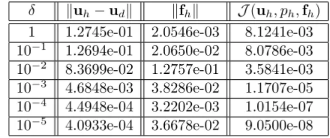
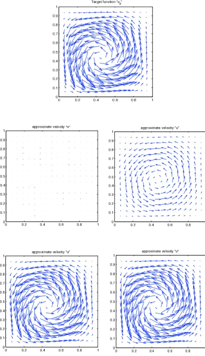
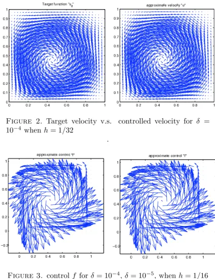
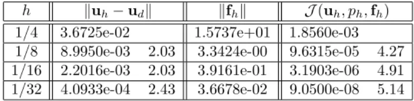
By choosing a parameter, we will show several computation results.

The plan of the paper is as follows. We introduce the notation and prelim-

inary results that will be used throughout the paper in the remainder of this

section. In §2, we give a precise statement of the optimization problem and

prove that an optimal solution exists. Then we reformulate the optimality sys-

tems to the first-order system and define the L ² and H ⁻¹ -norm least squares

functional. In §3, we obtain the optimal error estimates for least-squares finite

element method for the optimality system. Finally, In §4, some numerical tests

are performed.

1.1. Notation and preliminary results

The standard Sobolev spaces H ^m (Ω) and H ₀ ¹ (Ω) will be used with the as- sociated standard inner products (·, ·) m and their respective norms k · k m . In particular, for m = 0 we replace H ^m (Ω) by L ² (Ω) with the norm k · k and inner product (·, ·), and denote L ² ₀ (Ω) as the subspace of square integrable functions with zero mean. For positive values of m the space H ^−m (Ω) is defined as the dual space of H ₀ ^m (Ω) equipped with the norm kφk −m = sup _06=v∈H

0

(Ω) hφ,vi kvk

where h·, ·i is the duality pairing between H ^−m (Ω) and H ₀ ^m (Ω). Define the product spaces H ₀ ^m (Ω) ^d = Π ^d _i=1 H ₀ ^m (Ω) and H ^−m (Ω) ^d = Π ^d _i=1 H ^−m (Ω) with standard product norms. All subspaces are equipped with the norms inherited from the corresponding underlying spaces.

For an introduction of vorticity of the velocity u, we define the curl of v for a vector function v = (v 1 , v 2 ) ^t as the scalar function ∇ × v = ∂ x v 2 − ∂ y v 1 and denote by ∇ ^⊥ the formal adjoint of ∇× defined by ∇ ^⊥ p = (∂ _y p, −∂ _x p) ^t . Then with these notations it follows that

(1.5) ∇ ^⊥ ∇ × v = −∆v + grad div v.

Because the constrained optimal control problem is the present topic of this paper, we will make a lot use of the Stokes equations. First of all we recall the H ¹ regularity of the weak solutions of the Stokes equations. The weak form of the constraint equations (1.2)-(1.4) is then given as follows: seek u ∈ H ₀ ¹ (Ω) ² and p ∈ L ² ₀ (Ω) such that

νa(u, v) + b(v, p) = hf , vi ∀v ∈ H ₀ ¹ (Ω) ² , (1.6)

b(u, q) = 0 ∀q ∈ L ² ₀ (Ω), (1.7)

where h·, ·i is duality pairing and

a(u, v) = Z

Ω

∇u : ∇v dx, ∀u, v ∈ H ¹ (Ω) ² , b(u, q) = −

Z

Ω

q∇ · u dx ∀u ∈ H ¹ (Ω) ² , ∀q ∈ L ² (Ω).

Then, the (weak form of the) boundary value problem (1.6)-(1.7) is well-posed and has a unique solution (u, p) ∈ H ₀ ¹ (Ω) ² × L ² ₀ (Ω) for any f ∈ H ⁻¹ (Ω) ² (see [17]). The following stability condition is well known:

(1.8) kuk 1 + kpk ≤ Ckf k −1 ,

where C is a positive constant. From now on, a constant C will denote a

positive quantity whose meaning and values change with context.

2. Formulation and analysis of the optimal control problem 2.1. The optimization problem

We look for a (u, p, f ) ∈ H ₀ ¹ (Ω) ² × L ² ₀ (Ω) × H ⁻¹ (Ω) ² such that the cost functional

J (u, p, f ) = 1

2 ku − u d k ² + δ 2 kf k ² ,

subject to the constraints which are the stationary Stokes equations (1.2)-(1.4).

The admissibility set U ad is defined by

U ad = {(u, p, f ) ∈ H ₀ ¹ (Ω) ² × L ² ₀ (Ω) × H ⁻¹ (Ω) ² : (2.9)

J(u, p, f ) < ∞ and (u, p, f ) satisfies (1.6) and (1.7)}.

Then, (ˆ u, ˆ p, ˆf) is called an optimal solution if there exists an ² > 0 such that J (ˆ u, ˆ p, ˆf) ≤ J (u, p, f ) for all (u, p, f ) ∈ U ad satisfying ku − ˆ uk 1 + kp − ˆ pk + kf − ˆfk −1 ≤ ². The optimal control problem can now be formulated as a constrained minimization problem in a Hilbert space :

(2.10) min

(u,p,f )∈U

J (u, p, f ).

The existence and uniqueness of an optimal solution of (2.10) is easily proven using standard arguments in the following theorem.

Theorem 2.1. Given u d , there exists a unique solution (u, p, f ) ∈ U ad . Proof. We first note that U ad is clearly not empty. Let ©

(u ⁽ⁿ⁾ , p ⁽ⁿ⁾ , f ⁽ⁿ⁾ ) ª be a minimizing sequence, i.e., (u ⁽ⁿ⁾ , p ⁽ⁿ⁾ , f ⁽ⁿ⁾ ) ∈ U ad for all n and satisfies

n→∞ lim J (u ⁽ⁿ⁾ , p ⁽ⁿ⁾ , f ⁽ⁿ⁾ ) = inf

(u,p,f )∈U

J (u, p, f ).

Using the fact kf ⁽ⁿ⁾ k ² ≤ ² _δ J (u ⁽⁰⁾ , p ⁽⁰⁾ , f ⁽⁰⁾ ) and (1.8), we deduce that the sequence {ku ⁽ⁿ⁾ k 1 } and {kp ⁽ⁿ⁾ k} and {kf ⁽ⁿ⁾ k −1 } are uniformly bounded. So, we may then extract subsequences such that

f ⁽ⁿ

⁾ * ˜f in H ⁻¹ (Ω) ² , p ⁽ⁿ

⁾ * ˜ p in L ² ₀ (Ω), u ⁽ⁿ

⁾ * ˜ u in H ₀ ¹ (Ω) ² , u ⁽ⁿ

⁾ → ˜ u in L ² (Ω) ²

for some (˜ u, ˜ p, ˜f) ∈ H ₀ ¹ (Ω) ² × L ² ₀ (Ω) × H ⁻¹ (Ω) ² . The last convergence results above follows from the compact imbedding H ₀ ¹ (Ω) ² ,→,→ L ² (Ω) ² . By process of passing to the limit, we have that (˜ u, ˜ p, ˜f) satisfies (1.6)-(1.7). Now, by the weak lower semi-continuity of J (·, ·, ·), we conclude that (˜ u, ˜ p, ˜f) is an optimal solution, i.e.,

(u,p,f )∈U inf

J (u, p, f ) = lim

i→∞ inf J (u ⁽ⁿ

⁾ , p ⁽ⁿ

⁾ , f ⁽ⁿ

⁾ ) = J (˜ u, ˜ p, ˜f).

Thus, we have shown that an optimal solution belonging to U ad exists. Fi- nally, the uniqueness of the optimal solution follows from the convexity of the functional and the linearity of the constraint equations. ¤ 2.2. The optimality system

From the Lagrangian

L(u, p, f , v, q : u d ) = J (u, p, f ) − (ν∆u − ∇p + f , v) − (∇ · u, q), where J (·, ·, ·) is defined by (1.1), one may derive an optimality system of equations for the solution of (2.10). The constrained problem (2.10) can now be recast as the unconstrained problem of finding stationary points of L(·). We now apply the necessary conditions for the latter problem. Clearly, setting to zero the first variations with respect to u, p, f , v and q yields the optimality system

(2.11)

 

 

 

 

 



 

 

 

 

 

−ν∆u + ∇p = f in Ω,

∇ · u = 0 in Ω, u = 0 on ∂Ω,

−ν∆v + ∇q + u = u d in Ω,

∇ · v = 0 in Ω, v = 0 on ∂Ω, δf = v in Ω.

Note that this system is coupled, i.e., the constraint equations for the state vari- ables depend on the unknown controls, the adjoint equations for the Lagrange multipliers depend on the state, and optimality conditions for the controls de- pend on the Lagrange multipliers.

The strong form of the optimality system (2.11) may be written as first-order systems of partial differential equations by introducing meaningful variables ω = ∇ × u and z = ∇ × v. The formal normal for this first-order systems is not differentially diagonally dominant because of the optimality condition.

So, using the optimality condition f = ^v _δ , we obtain the following optimality system: find (ω, u, p, z, v, q) ∈ L ² (Ω) × H ₀ ¹ (Ω) ² × L ² ₀ (Ω) × L ² (Ω) × H ₀ ¹ (Ω) ² × L ² ₀ (Ω) such that

(2.12)

 

 

 

 

 

 

 



 

 

 

 

 

 

 

ν∇ ^⊥ ω + ∇p − v

δ = 0 in Ω,

∇ · u = 0 in Ω,

∇ × u − ω = 0 in Ω, u = 0 on ∂Ω, ν∇ ^⊥ z + ∇q + u = u d in Ω,

∇ · v = 0 in Ω,

∇ × v − z = 0 in Ω,

v = 0 on ∂Ω.

2.3. Least-squares functional

In this section, we discuss of the continuous H ⁻¹ and L ² least-squares func- tional on the space V where

V := L ² (Ω) × H ₀ ¹ (Ω) ² × L ² ₀ (Ω) × L ² (Ω) × H ₀ ¹ (Ω) ² × L ² ₀ (Ω) with a norm k| · k| as

k|(ω, u, p, z, v, q)k| = ¡

kωk ² + kuk ² ₁ + kpk ² + kzk ² + kvk ² ₁ + kqk ² ¢

2

. The proposed least-squares functional is defined by the L ² - and H ⁻¹ -norms of the residual equations of the system (2.12):

F(ω, u, p, z, v, q : u d ) = kν∇ ^⊥ ω + ∇p − v

δ k ² ₋₁ + k∇ · uk ² + kω − ∇ × uk ² + 1

δ ² kν∇ ^⊥ z + ∇q + u − u d k ² ₋₁ + 1

δ ² k∇ · vk ² + 1

δ ² kz − ∇ × vk ² . (2.13)

Note that the weight _δ ¹

is used for the balance of state and adjoint equations.

The least-squares problem we consider is to minimize this quadratic func- tional over V:

find (ω, u, p, z, v, q) ∈ V such that (2.14) F(ω, u, p, z, v, q : u d ) = inf

(τ,w,r,ψ,x,x)∈V F(τ, w, r, ψ, x, x : u d ).

In order to show the existence and uniqueness of the solutions of (2.14), the ellipticity and continuity of the proposed least-squares functional should be proven. One may note that the existence and uniqueness depends on δ and ν.

Theorem 2.2. For any (ω, u, p, z, v, q) ∈ V, there exist positive constant C 1 (δ, ν) and C 2 (δ, ν) such that

(2.15)

C 1 k|(ω, u, p, z, v, q)k| ² ≤ F(ω, u, p, z, v, q : 0) ≤ C 2 k|(ω, u, p, z, v, q)k| ² . Proof. The upper bound in (2.15) is straightforward from the triangle, Schwarz’

inequalities and definitions of H ⁻¹ -norm.

To prove the lower bound in (2.15), we modify the techniques in [12]. We assume that the domain Ω is simply connected. Using Green’s formula (see [17]), it follows that

1

δ k∇ × uk ² + 1

δ ² k∇ × vk ² (2.16)

= 1

δ (∇ × u − ω, ∇ × u) + 1

δ (ω, ∇ × u) + 1

δ ² (∇ × v − z, ∇ × v)+ 1

δ ² (z, ∇ × v)

= 1

δ (∇ × u − ω, ∇ × u) + 1

δ (∇ ^⊥ ω, u) + 1

δ ² (∇ × v − z, ∇ × v) + 1

δ ² (∇ ^⊥ z, v)

= 1

δ (∇ × u − ω, ∇ × u) + 1

νδ (ν∇ ^⊥ ω + ∇p − v

δ , u) + 1

νδ (p, ∇ · u) + ( 1

δ ∇ × v − 1 δ z, 1

δ ∇ × v) + 1 ν ( ν

δ ∇ ^⊥ z + 1 δ ∇q + 1

δ u, 1 δ v) + 1

νδ (q, 1 δ ∇ · v) and

1

δ kωk ² + 1 δ ² kzk ² (2.17)

= 1

δ (ω − ∇ × u, ω) + 1

δ (∇ × u, ω) + 1

δ ² (z − ∇ × v, z) + 1

δ ² (∇ × v, z)

= 1

δ (ω − ∇ × u, ω) + 1

δ (∇ ^⊥ ω, u) + 1

δ ² (z − ∇ × v, z) + 1

δ ² (∇ ^⊥ z, v)

= 1

δ (ω − ∇ × u, ω) + 1

νδ (ν∇ ^⊥ ω + ∇p − v

δ , u) + 1

νδ (p, ∇ · u) + ( 1

δ z − 1

δ ∇ × v, 1 δ z) + 1

ν ( ν

δ ∇ ^⊥ z + 1 δ ∇q + 1

δ u, 1 δ v) + 1

νδ (q, 1 δ ∇ · v).

Combining (2.16) and (2.17), using the ²-inequality and Schwarz’ inequality, we have

1

δ k∇ × uk ² + 1

δ ² k∇ × vk ² + 1

δ kωk ² + 1 δ ² kzk ² (2.18)

= 1

δ k∇ × u − ωk ² + 2

νδ (ν∇ ^⊥ ω + ∇p − v

δ , u) + 2

νδ (p, ∇ · u) + 1

δ ² k∇ × v − zk ² + 2 ν ( ν

δ ∇ ^⊥ z + 1 δ ∇q + 1

δ u, 1 δ v) + 2

νδ (q, 1 δ ∇ · v)

≤ 1

δ k∇ × u − ωk ² + 1

² 1 δ kν∇ ^⊥ ω + ∇p − v

δ k ² ₋₁ + ² 1

δν ² kuk ² ₁ + 2

νδ kpkk∇ · uk + 1

δ ² k∇ × v − zk ² + 1

² 2 k ν

δ ∇ ^⊥ z+ 1 δ ∇q+ 1

δ uk ² ₋₁ + ² 2

ν ² k 1

δ vk ² ₁ + 2 νδ kqkk 1

δ ∇ · vk.

For any φ ∈ H ₀ ¹ (Ω) ² we have

(∇p, φ) = (ν∇ ^⊥ ω + ∇p − v

δ , φ) − ν(ω, ∇ × φ) + 1 δ (v, φ)

≤ µ

kν∇ ^⊥ ω + ∇p − v

δ k −1 + νkωk + 1 δ kvk

¶ kφk 1 . Hence, using the fact kpk ≤ Ck∇pk −1 , we have

kpk ≤ C ^∗ µ

kν∇ ^⊥ ω + ∇p − v

δ k ₋₁ + νkωk + 1

δ k∇ × vk

¶ , (2.19)

where C ^∗ is independent of δ and ν. In a similar way, we have kqk ≤ C ^∗ ¡

kν∇ ^⊥ z + ∇q + uk −1 + νkzk + k∇ × uk ¢ , (2.20)

where C ^∗ is independent of ν.

Now from (2.18)-(2.20) and ²-inequality, we have 1

δ k∇ × uk ² + 1

δ ² k∇ × vk ² + 1

δ kωk ² + 1 δ ² kzk ²

≤ 1

δ k∇ × u − ωk ² + 1

δ² 1 kν∇ ^⊥ ω + ∇p − v

δ k ² ₋₁ + ² 1 C

δν ² k∇ × uk ² + ² 1 C

δν ² k∇ · uk ² + C ^∗

δ (² 3 kν∇ ^⊥ ω + ∇p − v

δ k ² ₋₁ + 1 ν ² ² 3

k∇ · uk ² + ² 4 kωk ² + 1

² 4 k∇ · uk ² + ² 5 k 1

δ ∇ × vk ² + 1

ν ² ² 5 k∇ · uk ² ) + 1

δ ² k∇ × v − zk ² + 1

² 2

k ν

δ ∇ ^⊥ z + 1 δ ∇q + 1

δ uk ² ₋₁ + ² 2 C ν ² k 1

δ ∇ × vk ² + ² 2 C ν ² k 1

δ ∇ · vk ² + C ^∗ (² 6 k ν

δ ∇ ^⊥ z + 1 δ ∇q + 1

δ uk ² ₋₁ + 1 ν ² ² 6 k 1

δ ∇ · vk ² + ² 7 k 1 δ zk ² + 1

² 7 k 1

δ ∇ · vk ² + ² 8

δ ² k∇ × uk ² + 1 ν ² ² 8 k 1

δ ∇ · vk ² ),

where C is independent of δ and ν. By collecting the same terms, it follows that

³ 1 δ − ² 1 C

δν ² − C ^∗ ² 8

δ ²

´

k∇ × uk ² +

³

1 − ² 2 C

ν ² − ² 5 C ^∗ δ

´ 1

δ ² k∇ × vk ² + ³ 1

δ − C ^∗ ² 4

δ

´

kωk ² + ³

1 − C ^∗ ² 7 ´ 1 δ ² kzk ²

≤ 1

δ k∇ × u − ωk ² + ³ 1

δ² 1 + ² 3 C ^∗ δ

´

kν∇ ^⊥ ω + ∇p − v δ k ² ₋₁ + ³ ² ₁ C

δν ² + C ^∗ δν ² ² 3 + C ^∗

δ² 4 + C ^∗ δν ² ² 5

´

k∇ · uk ² + k 1

δ ∇ × v − 1 δ zk ² + ³ 1

² 2 + ² 6 C ^∗ ´ k ν

δ ∇ ^⊥ z + 1 δ ∇q + 1

δ uk ² ₋₁ + ³ C² ₂

ν ² + C ^∗ ν ² ² 6 + C ^∗

² 7 + C ^∗ ν ² ² 8

´ k 1

δ ∇ · vk ² .

If we take ² 1 = ² 2 = _3C ^ν

, ² 3 = ² 6 = _ν ¹

, ² 4 = ² 7 = _3C ¹

, ² 5 = _3C ^δ

and ² 8 = _3C ^δ

, then

k∇ × uk ² + k∇ · uk ² + k∇ × vk ² + k∇ · vk ² + kωk ² + kzk ² (2.21)

≤ C ₁ ^∗ (δ, ν) F(ω, u, p, z, v, q : 0), where

C ₁ ^∗ (δ, ν) =

 

 

 



3 max{1, 3C + C ^∗ ν ² , 2

3 + C ^∗ + 3C ^∗2 + 3C ^∗2

δν ² } for δ ≤ 1, 3δ ² max{1, 3C + C ^∗

ν ² , 2

3 + C ^∗ + 3C ^∗2 + 3C ^∗2

δν ² } for δ ≥ 1.

Combining (2.19) and (2.20), we have

(2.22) kpk ² + kqk ² ≤ C ₁ ^∗∗ (δ, ν)F(ω, u, p, z, v, q : 0),

where C ₁ ^∗∗ (δ, ν) = Cδ ³ max{ν ² , 1} C ₁ ^∗ (δ, ν) for δ ≥ 1 and C ₁ ^∗∗ (δ, ν) = C max{ν ² , 1} C ₁ ^∗ (δ, ν)/δ ³ for δ ≤ 1.

Therefore, combining (2.21) and (2.22) yields the conclusion (2.15). The proof for general Ω, that is, when we assume only that ∂Ω is C ^1,1 , now follows by an argument similar to the proof of Theorem 3.7 in [17]. ¤

3. Finite element approximations

Using standard techniques of the calculus of variations one can show that a minimizer of (2.13) out of the space V necessarily satisfies the variational problem(Euler-Lagrange equation):

find (ω, u, p, z, v, q) ∈ V such that (3.23)

B(ω, u, p, z, v, q; ˜ ω, ˜ u, ˜ p, ˜ z, ˜ v, ˜ q) = F (˜ ω, ˜ u, ˜ p, ˜ z, ˜ v, ˜ q), ∀(˜ ω, ˜ u, ˜ p, ˜ z, ˜ v, ˜ q) ∈ V, where

B(ω, u, p, z, v, q; ˜ ω, ˜ u, ˜ p, ˜ z, ˜ v, ˜ q)

= (ν∇ ^⊥ ω + ∇p − v

δ , ν∇ ^⊥ ω + ∇˜ ˜ p − ˜ v

δ ) −1 + (∇ · u, ∇ · ˜ u) + (ω − ∇ × u, ˜ ω − ∇ × ˜ u) + 1

δ ² (ν∇ ^⊥ z + ∇q + u, ν∇ ^⊥ ˜ z + ∇˜ q + ˜ u) −1

+ 1

δ ² (∇ · v, ∇ · ˜ v) + 1

δ ² (z − ∇ × v, ˜ z − ∇ × ˜ v) and

F (˜ ω, ˜ u, ˜ p, ˜ z, ˜ v, ˜ q) = 1

δ ² (u d , ν∇ ^⊥ z + ∇˜ ˜ q + ˜ u) −1 .

We can easily verify that the bilinear form B(·; ·) is elliptic and continuous with respect to the norm k| · k| in V, i.e., there exist positive constants C 1 and C 2

such that

C 1 k|(˜ ω, ˜ u, ˜ p, ˜ z, ˜ v, ˜ q)k| ² ≤ B(˜ ω, ˜ u, ˜ p, ˜ z, ˜ v, ˜ q; ˜ ω, ˜ u, ˜ p, ˜ z, ˜ v, ˜ q) (3.24)

and

B(˜ ω, ˜ u, ˜ p, ˜ z, ˜ v, ˜ q; ˜ ω, ˜ u, ˜ p, ˜ z, ˜ v, ˜ q) ≤ C 2 k|(˜ ω, ˜ u, ˜ p, ˜ z, ˜ v, ˜ q)k| ² , ∀(˜ ω, ˜ u, ˜ p, ˜ z, ˜ v, ˜ q) ∈ V, (3.25)

where both C 1 and C 2 depend on δ and ν and the linear form F (·) is apparently continuous. Thus, by the Lax-Milgram lemma, there exists a unique solution (ω, u, p, z, v, q) ∈ V to the problem (3.23) and then may get the control f by the optimality condition f = ^v _δ if it is needed.

For the finite element approximation, let T h be a partition of the Ω into finite elements, i.e., Ω = S

K∈T

K with h = max{diam(K) : K ∈ T h }. Assume

that the triangulation T h is a quasi-uniform, i.e., it is regular and satisfies the

inverse assumption (see [16]). Let V h := W h × U h × P h × W h × U h × P h

be a finite element subspace of V with the following properties: there exist a constant C and integer r ≥ 1, s ≥ 1 and k ≥ 1, for any (ω, u, p, z, v, q) ∈ (H ^r (Ω) × H ^s+1 (Ω) ² × H ^k (Ω) × H ^r (Ω) ×H ^s+1 (Ω) ² × H ^k (Ω)) T

V and a pair (ω h , p h , z h , q h ) ∈ W h × P h × W h × P h such that

(3.26) inf

ψ

∈S

(kψ − ψ h k + hkψ − ψ h k 1 ) ≤ Ch ^r kψk r ,

where ψ is ω, p, z or q and the space S h is either W h or P h corresponding to ω h or p h , q h there exists a pair (u h , v h ) ∈ U h × U h such that

(3.27) inf

w

∈U

(kw − w h k + hkw − w h k 1 ) ≤ Ch ^s+1 kwk s+1 , where w is u or v.

Note that typical finite element spaces consisting of continuous piecewise polynomials with respect to quasi-uniform triangulations satisfy (3.26), (3.27).

Then, the finite element approximation to (3.23) becomes:

find (ω h , u h , p h , z h , v h , q h ) ∈ V h such that (3.28)

B(ω h , u h , p h , z h , v h , q h ; ˜ ω h , ˜ u h , ˜ p h , ˜ z h , ˜ v h , ˜ q h ) = F (˜ ω h , ˜ u h , ˜ p h , ˜ z h , ˜ v h , ˜ q h ),

∀(˜ ω h , ˜ u h , ˜ p h , ˜ z h , ˜ v h , ˜ q h ) ∈ V h . Theorem 3.1. Let (ω, u, p, z, v, q) ∈ V be the solution of the problem (3.23) and let (ω h , u h , p h , z h , v h , q h ) ∈ V h be the solution of the problem (3.28). Then we have

k|(ω, u, p, z, v, q) − (ω h , u h , p h , z h , v h , q h )k|

(3.29)

≤ C inf

(˜ ω

,˜ u

,˜ p

,˜ z

,˜ v

,˜ q

)∈V

k|(ω, u, p, z, v, q) − (˜ ω h , ˜ u h , ˜ p h , ˜ z h , ˜ v h , ˜ q h )k|

and, if (ω, u, p, z, v, q) ∈ H ^r (Ω) × H ^s+1 (Ω) ² × H ^k (Ω) × H ^r (Ω) ×H ^s+1 (Ω) ² × H ^k (Ω) for some r ≥ 1, s ≥ 1 and k ≥ 1, then also

(3.30)

k|(ω, u, p, z, v, q) − (ω h , u h , p h , z h , v h , q h )k|

≤ C(h ^2r kωk ² _r + h ^2s kuk ² _s+1 + h ^2k kpk ² _k + h ^2r kzk ² _r + h ^2s kvk ² _s+1 + h ^2k kqk ² _k )

, where C depends on δ, ν and the domain Ω and the ratio of the constants C 2

and C 1 in Theorem 2.2.

Proof. It is easy to show that the error (ω −ω h , u−u h , p−p h , z −z h , v −v h , q − q h ) is orthogonal to V h with respect to the bilinear form B(·; ·). Standard finite element analyses and (3.24)-(3.25) yield the error estimate (3.29) and the approximation properties (3.26), (3.27) leads to (3.30). ¤ Corollary 3.1. Let the hypotheses of Theorem 3.1 hold. Let the approximate control be defined by f h = v h

δ . Then

kf−f h k −1 ≤ ˜ C(h ^2r kωk ² _r +h ^2s kuk ² _s+1 +h ^2k kpk ² _k +h ^2r kzk ² _r +h ^2s kvk ² _s+1 +h ^2k kqk ² _k )

.

Proof. The result follows from (2.11) and (3.30). ¤

If we use continuous piecewise quadratic polynomials for the approximation of the velocity and continuous piecewise linear polynomials for the approxima- tions of the vorticity and pressure, i.e., r, s, k = 2, the we get the following error estimate

k|(ω, u, p, z, v, q) − (ω h , u h , p h , z h , v h , q h )k|

≤ Ch ² (kωk ² ₂ + kuk ² ₃ + kpk ² ₂ + kzk ² ₂ + kvk ² ₃ + kqk ² ₂ )

,

which is optimal with respect to the finite element functions used. (3.30) shows that error bounds for the velocity obtained here is the best approximation in the subspace U h , but one may see that the error estimates for the vorticity and pressure are one order less than the best approximation in the subspaces W h and P h . However, the use of a single approximating space for all variables simplifies the programming of the finite element methods.

Although the bilinear form B(·; ·) appears attractive from the point of view of stability and accuracy, its computation is not feasible because of the evaluation of the H ⁻¹ (Ω) ² inner product. Following [10], we can employ the H ⁻¹ (Ω) ² inner product using a computable operator T h . Let ˜ A h : H ⁻¹ (Ω) ² → U h

be the discrete solution operator w = ˜ A h g ∈ U h for the Dirichlet problem.

Assume that there is a symmetric positive definite preconditioner operator A h : H ⁻¹ (Ω) ² → U h for ˜ A h which is spectrally equivalent to ˜ A h . Then for a fixed positive constants γ, define

T h = h ² I h + γA h ,

where I h denotes the identity operator on U h . It is also known that the H ⁻¹ (Ω) ² inner product (·, ·) −1 can be replaced by the equivalent discrete inner product such that (T h ·, ·) (see [10]). Now, let us define the discrete counter- parts of the bilinear form B(·; ·) and the linear functional F (·) such that

B γ (ω, u, p, z, v, q; ˜ ω, ˜ u, ˜ p, ˜ z, ˜ v, ˜ q)

= (T h (ν∇ ^⊥ ω + ∇p − v

δ ), ν∇ ^⊥ ω + ∇˜ ˜ p − v ˜

δ ) + (∇ · u, ∇ · ˜ u) + (ω − ∇ × u, ˜ ω − ∇ × ˜ u) + 1

δ ² (T h (ν∇ ^⊥ z + ∇q + u), ν∇ ^⊥ z + ∇˜ ˜ q + ˜ u) + 1

δ ² (∇ · v, ∇ · ˜ v) + 1

δ ² (z − ∇ × v, ˜ z − ∇ × ˜ v) and

F γ (˜ ω, ˜ u, ˜ p, ˜ z, ˜ v, ˜ q) = 1

δ ² (T h (u d ), ν∇ ^⊥ z + ∇˜ ˜ q + ˜ u).

Then, the discrete variational problem corresponding to (3.23) becomes:

find (ω h , u h , p h , z h , v h , q h ) ∈ V h such that

(3.31) B γ (ω h , u h , p h , z h , v h , q h ; ˜ ω, ˜ u, ˜ p, ˜ z, ˜ v, ˜ q) =F γ (˜ ω, ˜ u, ˜ p, ˜ z, ˜ v, ˜ q),

∀(˜ ω, ˜ u, ˜ p, ˜ z, ˜ v, ˜ q) ∈ V h .

A simpler approach to compute the H ⁻¹ (Ω) ² inner product is to use a scale argument (see [5]) which replaces kν∇ ^⊥ ω + ∇p − ^v _δ k ² ₋₁ by the weighted L ² (Ω) ² -norm h ² kν∇ ^⊥ ω + ∇p − ^v _δ k ² instead of the discrete negative norm

¡ T h (ν∇ ^⊥ ω + ∇p − ^v _δ ), ν∇ ^⊥ ω + ∇˜ ˜ p − ^{˜ v} _δ ¢

. This is nothing but to take γ = 0 in the problem (3.31), i.e., we take T h = h ² I h . Then, we have

B 0 (ω, u, p, z, v, q; ˜ ω, ˜ u, ˜ p, ˜ z, ˜ v, ˜ q)

= h ² (ν∇ ^⊥ ω + ∇p − v

δ , ν∇ ^⊥ ω + ∇˜ ˜ p − v ˜

δ ) + (∇ · u, ∇ · ˜ u) + (ω − ∇ × u, ˜ ω − ∇ × ˜ u) + h ²

δ ² (ν∇ ^⊥ z + ∇q + u, ν∇ ^⊥ z + ∇˜ ˜ q + ˜ u) + 1

δ ² (∇ · v, ∇ · ˜ v) + 1

δ ² (z − ∇ × v, ˜ z − ∇ × ˜ v) and

F 0 (˜ ω, ˜ u, ˜ p, ˜ z, ˜ v, ˜ q) = h ²

δ ² (u d , ν∇ ^⊥ z + ∇˜ ˜ q + ˜ u).

The discrete problem B 0 (ω h ,u h , p h , z h , v h , q h ; ˜ ω,˜ u, ˜ p, ˜ z, ˜ v, ˜ q) = F 0 (˜ ω, ˜ u, ˜ p, ˜ z, ˜ v, ˜ q) is equivalent to a linear algebraic system:

(3.32)



 

 

 



K 1 C ^T ₁ C ^T ₂ 0 C ^T ₄ 0 C 1 K 2 0 C ^T ₃ 0 C ^T ₆ C 2 0 K 3 0 C ^T ₅ 0

0 C 3 0 K ^∗ ₁ C ^∗ ₁ ^T C ^∗ ₂ ^T C 4 0 C 5 C ^∗ ₁ K 4 0

0 C 6 0 C ^∗ ₂ 0 K ^∗ ₃



 

 

 





 

 

 



~ω

~u

~p

~z

~v

~q



 

 

 



=



 

 

 

 0

~f 0

~g 0

~h



 

 

 

 .

Indeed, we chooses bases {W i } ^m _i=1 , {U i } ⁿ _i=1 and {P i } ^r _i=1 for W h , U h , and P h , respectively, and we then have ω h = P _m

i=1 ω i W i , u h = P _n

i=1 u i U i , p h = P _r

i=1 p i P i , z h = P _m

i=1 z i W i, v h = P _n

i=1 v i U i and q h = P _r

i=1 q i P i for some sets of coefficients {ω i } ^m _i=1 , {u i } ⁿ _i=1 , {p i } ^r _i=1 , {z i } ^m _i=1 , {v i } ⁿ _i=1 and {q i } ^r _i=1 that are determined by solving (3.32). In (3.32), we have that ~ω = (ω 1 , . . . , ω m ) ^T ,

~u = (u 1 , . . . , u n ) ^T , ~p = (p 1 , . . . , p r ) ^T , ~z = (z 1 , . . . , z m ) ^T , ~v = (v 1 , . . . , v n ) ^T and

~q = (q 1 , . . . , q r ) ^T ,

(K 1 ) ij = h ² ν ² (∇ ^⊥ W j , ∇ ^⊥ W i ) + (W j , W i ) for i, j = 1, . . . , m (K ^∗ ₁ ) ij = h ² ν ²

δ ² (∇ ^⊥ W j , ∇ ^⊥ W i ) + 1

δ ² (W j , W i ) for i, j = 1, . . . , m (K 2 ) ij = (∇ · U j , ∇ · U i ) + (∇ × U j , ∇ × U i ) + h ²

δ ² (U j , U i ) for i, j = 1, . . . , n (K 3 ) ij = h ² (∇P j , ∇P i ) for i, j = 1, . . . , r

(K ^∗ ₃ ) ij = h ²

δ ² (∇P j , ∇P i ) for i, j = 1, . . . , r (K 4 ) ij = 1

δ ² (∇ · U j ,∇ · U i )+ 1

δ ² (∇ × U j ,∇ × U i )+ h ²

δ ² (U j , U i ) for i, j = 1, . . . , n

(C 1 ) ij = −(W j , ∇ × U i ) for i = 1, . . . , n, j = 1, . . . , m (C ^∗ ₁ ) ij = − 1

δ ² (W j , ∇ × U i ) for i = 1, . . . , n, j = 1, . . . , m (C 2 ) ij = h ² ν(∇ ^⊥ W j , ∇P i ) for i = 1, . . . , r, j = 1, . . . , m (C ^∗ ₂ ) ij = h ² ν

δ ² (∇ ^⊥ W j , ∇P i ) for i = 1, . . . , r, j = 1, . . . , m (C 3 ) ij = h ² ν

δ ² (U j , ∇ ^⊥ W i ) for i = 1, . . . , m, j = 1, . . . , n (C 4 ) ij = − h ² ν

δ (∇ ^⊥ W j , U i ) for i = 1, . . . , n, j = 1, . . . , m (C 5 ) ij = − h ²

δ (∇P j , U i ) for i = 1, . . . , n, j = 1, . . . , r (C 6 ) ij = h ²

δ ² (U j , ∇P i ) for i = 1, . . . , r, j = 1, . . . , n (~f) i = h ²

δ ² (u d , U i ) for i = 1, . . . , n (~g) i = h ² ν

δ ² (u d , ∇ ^⊥ W i ) for i = 1, . . . , m (~h) i = h ²

δ ² (u d , ∇P i ) for i = 1, . . . , r.

Remark 3.1. It easily follows from Theorem 2.2 that the coefficient matrix in (3.32) is symmetric and positive definite. Moreover, all four coefficient matri- ces K 1 , K ^∗ ₁ , K 2 , K 3 , K ^∗ ₃ , and K 4 of the linear systems in (3.32) are themselves symmetric and positive definite.

4. Numerical experiments

In this section, we present computational study of the problem (3.32) in a unit square domain Ω = (0, 1) × (0, 1) ⊂ R ² . The domain Ω is triangulized uni- formly with the grid interval h ranging from 2 ⁻² to 2 ⁻⁵ for each direction. We use the single approximating space of continuous piecewise linear polynomials for the approximations of all unknowns. Although our analysis does not in- clude the error estimate in that case, we expect to observe rates of convergence O(h ² ) for the L ² error ku − u d k.

The norms are all discrete norms measured by the five-point Gaussian quad- rature rule in each triangle based on the triangulation T h . We use the multigrid V-cycle method with the Gauss-Seidel smoothing iteration. We set the toler- ance of the errors to be 10 ⁻⁴ and the maximum number of iterations to be 300.

We tested the problem with the following simple desired state (target velocity) u _d (x, y) = (u(x, y), v(x, y)) is chosen where

u = d

dy φ(x)φ(y) and v = − d

dx φ(x)φ(y)

Table 1. The norms ku h − u d k, kf h k and J(u h , p h , f h ) when h = 1/16.

δ ku h − u d k kf h k J (u h , p h , f h ) 1 1.2745e-01 2.0007e-03 8.1239e-03 10 ⁻¹ 1.2682e-01 1.9950e-02 8.0610e-03 10 ⁻² 8.5708e-02 1.3286e-01 3.7612e-03 10 ⁻³ 6.6866e-03 4.9484e-02 2.3580e-05 10 ⁻⁴ 2.2184e-03 4.4086e-02 2.5578e-06 10 ⁻⁵ 2.2016e-03 3.9161e-01 3.1903e-06

Table 2. The norms ku h − u d k, kf h k and J(u h , p h , f h ) when h = 1/32.

δ ku h − u d k kf h k J (u h , p h , f h ) 1 1.2745e-01 2.0546e-03 8.1241e-03 10 ⁻¹ 1.2694e-01 2.0650e-02 8.0786e-03 10 ⁻² 8.3699e-02 1.2757e-01 3.5841e-03 10 ⁻³ 4.6848e-03 3.8286e-02 1.1707e-05 10 ⁻⁴ 4.4948e-04 3.2202e-03 1.0154e-07 10 ⁻⁵ 4.0933e-04 3.6678e-02 9.0500e-08

and

φ(z) = (1 − z) ² (1 − cos(πz)).

The initial velocity and adjoint variable are set to zeros. We examine the effects of changes in the penalty parameter δ. To show the effects of the δ, we report the discrete L ² -norm distances between the desired states u d and controlled state u h , the norm of control f h and the value of the cost functional J. All computations were carried out with ν = 1.

In Table 1, we present numerical results for the cases δ = 1, 10 ⁻¹ , 10 ⁻² , and

so on. For the case h = 1/16, we see that the L ² error ku _h − u _d k goes to

zero as δ goes to zero. Table 2 shows the numerical results when h = 1/32

is fixed. We have a phenomenon similar to those of Table 1. Figures 1 and

2 illustrate that the numerical solution u h converging to target velocity u d .

In Figure 1, we display the target velocity and approximate velocities for δ =

10 ⁻¹ , 10 ⁻² , 10 ⁻³ , 10 ⁻⁴ when h = 1/16 is fixed. In Figure 2, the approximate

velocity u h is similar to the target velocity u d for δ = 10 ⁻⁴ when h = 1/32 is

fixed. Figure 3 show the graph of control f for δ = 10 ⁻⁴ , 10 ⁻⁵ when h = 1/16

is fixed.

Figure 1. Target velocity u d (top), controlled velocities for

different values of δ; δ = 10 ⁻¹ , 10 ⁻² , 10 ⁻³ , 10 ⁻⁴ (from top to

bottom and left to right) when h = 1/16.

Figure 2. Target velocity v.s. controlled velocity for δ = 10 ⁻⁴ when h = 1/32

.

Figure 3. control f for δ = 10 ⁻⁴ , δ = 10 ⁻⁵ , when h = 1/16 Table 3. The norms ku _h − u _d k, kf _h k and J(u _h , p _h , f _h ) with convergence rate for δ = 10 ⁻⁴ .

h ku h − u d k kf h k J (u h , p h , f h ) 1/4 3.6726e-02 1.5375e-00 7.9258e-04 1/8 8.9823e-03 2.03 3.3640e-01 4.5999e-05 4.11 1/16 2.2184e-03 2.02 4.4086e-02 2.5578e-06 4.17 1/32 4.4948e-04 2.30 3.2202e-03 1.0154e-07 4.65

For the cases δ = 10 ⁻⁴ , 10 ⁻⁵ , Tables 3 and 4 show the numerical results

with convergence rates. Table 3 shows the discretization approximate error

Table 4. The norms ku h − u d k, kf h k and J(u h , p h , f h ) with convergence rate for δ = 10 ⁻⁵ .

h ku h − u d k kf h k J (u h , p h , f h ) 1/4 3.6725e-02 1.5737e+01 1.8560e-03 1/8 8.9950e-03 2.03 3.3424e-00 9.6315e-05 4.27 1/16 2.2016e-03 2.03 3.9161e-01 3.1903e-06 4.91 1/32 4.0933e-04 2.43 3.6678e-02 9.0500e-08 5.14

bound of ku h − u d k and J(u h , p h , f h ) are like O(h ² ) and O(h ⁴ ), respectively.

In Table 4, we have the numerical results similar to those of Table 3. But the norm of control f of Table 4 is a little larger than that of Table 3. In the case of δ = 1, 10 ⁻¹ , . . . , 10 ⁻³ , we don’t have the predicted error bound. In this point of view, the choice of δ = 10 ⁻⁴ seems to be the best choice among the present result for fixed ν = 1.

References

[1] H. K. Baek, S. D. Kim, and H.-C. Lee, A Multigrid method for an optimal control problem of a diffusion-convection equation, submitted.

[2] M. Bergounioux, Augmented Lagrangian method for distributed optimal control problems with state constraints, J. Optim. Theory Appl. 78 (1993), no. 3, 493–521.

[3] P. B. Bochev and M. D. Gunzburger, Analysis of least squares finite element methods for the Stokes equations, Math. Comp. 63 (1994), no. 208, 479–506.

[4] , Least-squares methods for the velocity-pressure-stress formulation of the Stokes equations, Comput. Methods Appl. Mech. Engrg. 126 (1995), no. 3-4, 267–287.

[5] , Finite element methods of least-squares type, SIAM Rev. 40 (1998), no. 4, 789–837.

[6] , Least-squares finite-element methods for optimization and control problems for the Stokes equations, Comput. Math. Appl. 48 (2004), no. 7-8, 1035–1057.

[7] , Least-squares finite element methods for optimality systems arising in opti- mization and control problems, SIAM J. Numer. Anal. 43 (2006), no. 6, 2517–2543.

[8] P. B. Bochev, T. A. Manteuffel, and S. F. McCormick, Analysis of velocity-flux first- order system least-squares principles for the Navier-Stokes equations. I., SIAM J. Nu- mer. Anal. 35 (1998), no. 3, 990–1009.

[9] , Analysis of velocity-flux least-squares principles for the Navier-Stokes equa- tions. II., SIAM J. Numer. Anal. 36 (1999), no. 4, 1125–1144.

[10] J. H. Bramble, R. D. Lazarov, and J. E. Pasciak, A least-squares approach based on a discrete minus one inner product for first order systems, Math. Comp. 66 (1997), no.

219, 935–955.

[11] J. H. Bramble and J. E. Pasciak, Least-squares methods for Stokes equations based on a discrete minus one inner product, J. Comput. Appl. Math. 74 (1996), no. 1-2, 155–173.

[12] Z. Cai, T. Manteuffel, and S. McCormick, First-order system least squares for velocity- vorticity-pressure form of the Stokes equations, with application to linear elasticity, Electron. Trans. Numer. Anal. 3 (1995), Dec., 150–159.

[13] , First-order system least squares for the Stokes equations, with application to linear elasticity, SIAM J. Numer. Anal. 34 (1997), no. 5, 1727–1741.

[14] C. Chang and M. Gunzburger, A finite element method for first order elliptic systems

in three dimensions, Appl. Math. Comput. 23 (1987), no. 2, 171–184.

[15] Y. Choi, H.-C. Lee, and B.-C. Shin, A least-squares/penalty method for distributed optimal control problems for Stokes equations, Comput. Math. Appl. 53 (2007), no. 11, 1672–1685.

[16] P. Ciarlet, The Finite Element Method for Elliptic Problems, Studies in Mathemat- ics and its Applications, Vol. 4. North-Holland Publishing Co., Amsterdam-New York- Oxford, 1978.

[17] V. Girault and P.-A. Raviart, Finite Element Methods for Navier-Stokes Equations, Theory and algorithms. Springer Series in Computational Mathematics, 5. Springer- Verlag, Berlin, 1986.

[18] R. Glowinski and J. He, On shape optimization and related issues, Computational meth- ods for optimal design and control (Arlington, VA, 1997), 151–179, Progr. Systems Con- trol Theory, 24, Birkhauser Boston, Boston, MA, 1998.

[19] M. D. Gunzburger, Perspectives in Flow Control and Optimization, Advances in Design and Control, 5. Society for Industrial and Applied Mathematics (SIAM), Philadelphia, PA, 2003.

[20] M. D. Gunzburger, L. S. Hou, and T. Svobodney, Analysis and finite element approx- imation of optimal control problems for the stationary Navier-Stokes equations with distributed and Neumann controls, Math. Comp. 57 (1991), no. 195, 123–151.

[21] M. D. Gunzburger and H.-C. Lee, Analysis and approximation of optimal control prob- lems for first-order elliptic systems in three dimensions, Appl. Math. Comput. 100 (1999), no. 1, 49–70.

[22] , A penalty/least-squares method for optimal control problems for first-order el- liptic systems, Appl. Math. Comput. 107 (2000), no. 1, 57–75.

[23] J.-W. He, R. Glowinski, R. Metcalfe, A. Nordlander, and J. Periaux, Active control and drag optimization for flow past a circular cylinder, J. Comput. Phys. 163 (2000), no. 1, 83–117.

[24] J.-W. He, M. Chevalier, R. Glowinski, R. Metcalfe, A. Nordlander, and J. Periaux, Drag reduction by active control for flow past cylinders, Computational mathematics driven by industrial problems (Martina Franca, 1999), 287–363, Lecture Notes in Math., 1739, Springer, Berlin, 2000.

[25] B.-N. Jiang and L. A. Povinell, Optimal least-squares finite element method for elliptic problems, Comput. Methods Appl. Mech. Engrg. 102 (1993), no. 2, 199–212.

[26] H.-C. Lee and Y. Choi, A least-squares method for optimal control problems for a second- order elliptic system in two dimensions, J. Math. Anal. Appl. 242 (2000), no. 1, 105–128.

[27] H.-C. Lee and O. Yu. Imanuvilov, Analysis of Neumann boundary optimal control prob- lems for the stationary Boussinesq equations including solid media, SIAM J. Control Optim. 39 (2000), no. 2, 457–477.

[28] , Analysis of optimal control problems for the 2-D stationary Boussinesq equa- tions, J. Math. Anal. Appl. 242 (2000), no. 2, 191–211.

Youngmi Choi

Department of Mathematics Ajou University

Suwon 443-749, Korea

E-mail address: ymchoi93@hanmail.net, ymchoi93@ajou.ac.kr

Sang Dong Kim

Department of Mathematics Kyungpook National University Daegu 702-701, Korea

E-mail address: skim@knu.ac.kr

Hyung-Chun Lee

Department of Mathematics Ajou University

Suwon 443-749, Korea

E-mail address: hclee@ajou.ac.kr