Numerical Study on the Correction of Sea Effect in Magnetotelluric (MT) Data

Numerical Study on the Correction of Sea Effect in Magnetotelluric (MT) Data

Junmo Yang

and Hai-Soo Yoo

Korea Ocean Research and Development Institute, Gyeonggi 425-600, Korea

Abstract: When magnetotelluric (MT) data are obtained in the vicinity of the coast, the surrounding seas make it difficult to interpret subsurface structure, especially the deep part of the subsurface. We introduce an iterative method to correct the sea effect, based on the previous topographic correction method that removes the distortion due to topographic changes in seafloor MT data. The method first corrects the sea effect in observed MT impedance, and then inverts corrected response in a model space without the sea. Due to mutual coupling between the sea and the subsurface structure, the correction and inversion steps are iterated until the changes in each result become negligible. The method is tested for 1- and 2-D structures using synthetic MT data produced by 3-D forward modeling including surrounding seas.

In all cases, the method closely recovers the true structure assumed to generate synthetic responses after a few iterations.

Keywords: mangetotelluric (MT), sea effect, correction of the sea effect

Introduction

A number of magnetotelluric (MT) survey have been extensively carried out since the 1970s to delineate electrical conductivity structure of subsurface of the Earth. In recent years, its target area has been extended to diverse tectonic settings, including seafloor environment such as marginal basins, subduction systems, and mid-ocean ridges (Filloux, 1977;

Wannermaker et al., 1989; Nolasco et al., 1998; Evans et al., 1999; Santos et al., 2001; Koyama, 2002; Baba et al., 2006). As data quality improves with the advance of measurement instrument and processing technique, main interest has been focusing more on accurate and reliable interpretation of earth structure in increasingly complex situations.

Generally, MT survey aims to figure out regional geoelectrical structure and conductivity anomalies of subsurface. However, the observed MT responses can be severely distorted by a variety of causes; artificial noises around observation site, near-surface conductivity inhomogeneity, complex topography, surrounding seas, and so forth. The effect of artificial noises has been

effectively reduced in MT data processing by the development of remote reference technique (Gamble et al., 1979) and various robust processing techniques (Egbert and Booker, 1986; Chave and Thomson, 1989;

Egbert, 1997; Chave and Thomson, 2004). Distortions in electromagnetic fields due to near-surface inhomogeneity have been successfully eliminated using tensor decomposition techniques (Groom and Bailey, 1989; Mcneice and Jones, 2001) in spite of inherent limitations of physical model assumed. Since Wannamaker et al. (1986) initially proposed the topographic correction method for 2-D structure, many researchers have presented various correction methods.

Recently, Nam (2006) has developed the topographic correction method for 3-D structure using edge finite element method. As a number of seafloor MT survey have been performed since the late of 1990s, studies on the correction method that removes distortions from island and bathymetry have been actively performed as well (Nolasco et al., 1998; Koyama, 2002; Baba and Chave, 2005).

Studies on sea effect correction have been carried out especially in geomagnetic depth sounding (Weaver and Agarwal, 1991; Bapat et al., 1993; Dosso et al., 1996; Shimoizumi et al., 1997; Pringle et al., 2000;

Yang, 2006). In these studies, 3-D forward modeling was performed to estimate the effect of surrounding

*Corresponding author: [email protected] Tel: 82-31-400-7687

Fax: 82-31-400-6147

Numerical Study on the Correction of Sea Effect in Magnetotelluric (MT) Data

551 seas and then sea effect was compared with observed

or corrected responses in terms of induction arrow. In MT survey, Nolasco et al. (1998) initially tried to correct sea effect in Society Island seafloor MT data employing electrical and magnetic distortion tensor.

Since they used 3-D thin-sheet modeling over 1-D mantle, there is a limitation that the subsurface structure should be 1-D. Similar to Nalasco et al.

(1998), Santos et al. (2001) have also corrected sea effect in land MT data using Mackie et al.’s 3-D forward algorithm. But the subsurface structure assumed in forward modeling should be precisely determined as prior information. Until now, correction of sea effect remains a serious challenge in the interpretation of land MT data.

The Korean Peninsula is surrounded by the sea on three sides. The surrounding seas severely affect observed MT responses even in the region largely separated from the coast due to sharp contrast between the sea and land in electrical property. In general, this is called “sea effect”, which make it difficult to determine the geoelectrical structure, especially that of deep part of the subsurface. Basically, frequency and separation distance where the sea effect starts to appear depend on the electrical structure of the subsurface (Bailey, 1977; Weaver and Dawson, 1992).

In order to accurately correct the sea effect, we need to know the electrical structure of the subsurface.

However, it can not be precisely determined without the sea effect correction. This leads us to a dilemma.

To solve this dilemma, Koyama (2002) and Baba and Chave (2005) have suggested an iterative method correcting distortions due to the change of bathymetry in seafloor voltage and MT data, respectively.

Their iterative method is composed of two stages.

First stage corrects the topographic effects in observed responses based on the initial subsurface structure.

Second stage inverts corrected responses in an appropriate model space without topography. The correction phase requires an assumed subsurface structure, and hence topographic correction is principally dependent on the resulting inverted model.

This nonlinear dependence may be handled iteratively;

correction phase is carried out again using subsurface structure updated from inversion phase at the previous iteration until neither the topographic correction nor the inverted model change significantly. Since this method is an iterative procedure, we do not need to take account into mutual coupling between the subsurface structure and topography. In addition, it can be applied to diverse tectonic settings regardless of the dimensionality of the subsurface. Therefore, this method can be a reasonable alternative for correcting the sea effect in land MT data. In this study, an iterative sea effect correction method is proposed and then verified for an 1-D and 2-D structure using synthetic MT data produced by 3-D forward modeling

The Correction Method

The method proposed in this paper is based on iteration between two stages suggested by Koyama (2002) and Baba and Chave (2005). We apply this iterative method to correct the sea effect in land MT data with a slight modification. The first stage is the correction of the sea effect in the observed MT responses and the second stage is the inversion of the corrected responses for a suitable subsurface structure.

The procedure can be summarized as follow.

(1) Correction phase: the MT response of a subsurface model with and without 3-D sea is numerically calculated, and the sea effect is estimated. The sea effect is then removed from observed MT responses.

(2) Inversion phase: the corrected MT response is inverted for structure using any suitable model at the appropriate dimensionality. The model space for inversion does not include the sea since the MT response is corrected to space without the sea.

Since the sea effect correction phase requires an

assumption for a subsurface structure, this process is

basically dependent on the inversion result. This

nonlinear dependence can be treated iteratively

identical to the topographic correction described

previously. Thus, correction and inversion phase is

iterated until neither the topographic correction nor the inverted model change significantly. The final result is typically insensitive to the initial subsurface model.

The simplest and most objective choice is a half-space model, although more complicated situations may easily be accommodated.

Correction of the MT impedance tensor is achieved by assuming a theoretical relationship

Z

=

(1)

where

is the MT response which includes the influence of the sea,

is a tensor describing the sea effect, and

is the response to subsurface structure without the sea. This relationship was introduced by Heison and Lilley (1993), although the approximation that

is 1-D was applied. In this study, all elements in Eq. (1) are complex 2×2 tensors and

may be the response to a 2-D or 3-D structure, and hence the method can be applied in any tectonic setting. Note that this multiplicative relation is similar to that for galvanic decomposition except that

becomes real rather than complex, and ultimately flows from an integral equation description of electromagnetic distortion, as derived by Groom and Barh (1992) and Chave and Smith (1994).

can be estimated from 3- D forward modeling of

and

. The subsurface structure must be given as a priori in the initial stage of solution. Once

is obtained, we can correct the observed MT response,

. Applying Eq. (1) to

and rearranging yields

Zc

=

(2)

where

is the response corrected for the sea effect that corresponds to the theoretical entity

. In practice, we can calculate from the observed MT response (

) and the modeled responses (

and

) while skipping the calculation of

to give

Zc

=

=(

)

=

(3)

is then inverted in a model space without the sea. In the subsequent stages of the solution, the model obtained from inversion of

is used to recorrect

. The iterative solution terminates under

any suitable criterion. We have adopted the root mean square (RMS) misfit between

and

in the domain of log apparent resistivity, log

, and phase,

,

RMS= (4)

where

log

and

are estimated errors in log apparent resistivity and phase, and is the number of data. If the RMS misfit change is below a threshold value (5% in this study), the iteration is terminated. In addition, since the subsurface structure used in this study is limited to 1D or 2-D and diagonal components of MT impedance tensor produced by 3-D forward modeling is very small, Eq. (3) can be reduced to simpler form (See Baba and Chave, 2005, for the details).

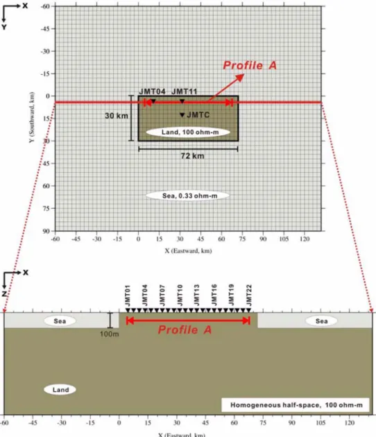
Verification with Synthetic MT Data Homogeneous half-space with 3-D sea (Model A) To verify the correction method proposed, we built a simple 3-D model that consists of 3-D sea over a homogeneous half-space (Model A). A 3-D staggered finite difference algorithm (Mackie et al., 1993) was employed for generating synthetic MT data. The geometry of the model is a simplified version to that of the Jeju Island, Korea, and the thickness of surrounding sea is set to 100m for the convenience of modeling (Fig. 1). The total nodes of the Model A are 78 (X, EW)

64 (Y, NS)

49 (Z, including 12 air layers) grids but the core of the model is composed of 64 (X, EW)

50 (Y, NS) grids with a 3 km spacing.

The outer grids of the core are used for 2-D extension adding 7 grids for each horizontal direction. Synthetic MT responses were generated for 20 frequencies equally spaced on a log scale between 10

and 10

Hz. A 100

·

half-space is given as the subsurface resistivity, and the resistivity of the sea is set to 0.33

·

.

1-D inversion:

We first demonstrate the iterative sea effect correction and 1-D inversion for synthetic

2N1

--- log ρ( oi⁄ρi) δlogρoi

--- ² φoi–φi

δφoi

--- ²

⎩ + ⎭

⎨ ⎬

⎧ ⎫

i 1= N

∑

Numerical Study on the Correction of Sea Effect in Magnetotelluric (MT) Data

553

MT data obtained from the Model A. In 1-D inversion, effective impedance is generally used to reduce the unwanted galvanic and inductive distortions (Likelybrooks, 1986; Berdichevsky et al., 1989). In this study, we have employed the determinant of MT impedance tensor defined as Eq. (5).

(5)

is rotationally invariant and frequently used to estimate the average 1-D structure. There are other

effective impedances such as arithmetic or geometric average of off-diagonal terms but they will give similar results. The Occam 1-D inversion method of Constable et al. (1987) is applied to the apparent resistivity and phase for

with 3% error floor. The initial model used in the inversion is set to 100

·

half-space. Fig. 2 shows observed MT responses and 1-D inverted models at sites JMT04, JMT11, and JMTC. Since the assumed subsurface structure is a 100

·

half-space, apparent resistivity and phase in

Zdet= ZxxZyy–ZxyZyx

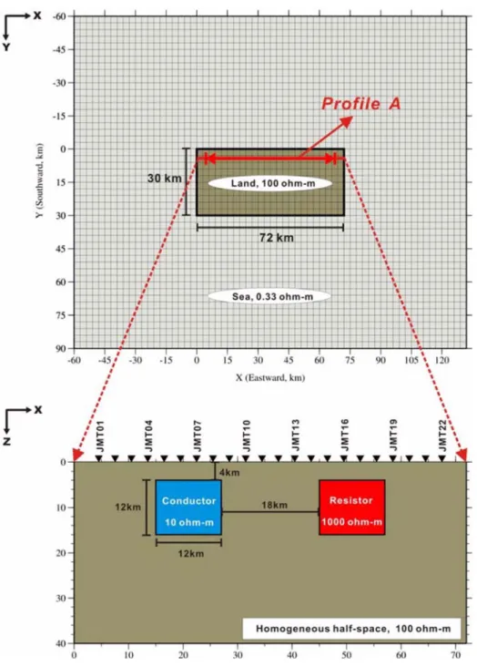
Fig. 1. 3-D model for correction of sea effect (Model A). In upper panel, the spacing of each grid is set to 3 km.

the absence of the sea should be a constant 100

·

and a 45 degree, respectively. But the MT response at each site differ from that of the half-space due to the effect of the sea, showing minimum for apparent resistivity and maximum for phase at frequencies ranging from 1 to 0.1 Hz. At site JMTC, which is located at the center of the island, the sea effect appears at lower frequency. The models obtained by 1-D inversion also show a similar pattern, as can be easily expected from the responses. A boundary between layers appears at about 5-10 and 30-40 km for all sites. This artificial feature may be erroneously interpreted as real geological structures.

We now demonstrate the sea effect correction example for synthetic data obtained from site JMT04.

The details for the correction step are described as follow.

(1) Add 3% random noise to

calculated from synthetic data and set it as

.

(2) Calculate

and

using 3-D forward modeling, based on 1-D model fit of uncorrected MT response (

)

(3) Correct

and estimate

, using Eq. (3) (4) Perform 1-D inversion to for a model space

without the sea

(5) Calculate

and

using 3-D forward modeling, based on the 1-D model fit updated by inversion of

.

The procedure from the step (3) to (5) is iterated until RMS misfit between

and

change become smaller than a given threshold value. Figure 3 shows the 1-D inverted model and RMS misfit at each iteration stage. The initial RMS misfit is 2.4 and it converged to 0.3 after 3 iterations. Actually, discrepancy

Fig. 2. (a) Apparent resistivity and phase for the square root of the determinant of the MT tensor (circles, diamonds, and trian- gles for sites JMT04, JMT11, and JMTC, respectively), along with the fit of a 1-D model to them (solid, dashed, and dotted lines, respectively). (b) 1D inverted models obtained by Occam inversion of the determinant of impedance tensor at each site.

Numerical Study on the Correction of Sea Effect in Magnetotelluric (MT) Data

555

between inverted models at the second and third iteration stage is very small. The final model is a half- space of 104

·

, and hence the subsurface structure assumed in forward modeling is successfully recovered. The tests for other sites showed similar results, although they are not displayed in Fig. 3.

2-D inversion:

We now test the sea effect correction method for a 2-D subsurface structure. For obtaining 2-D profile MT data, synthetic responses are calculated at 22 sites along profile A in the Model A (Fig. 1).

The strike direction is assumed to the y axis. The leftmost site is named as JMT01 and the rightmost one JMT22 with a 3 km spacing. The sites JMT01 and JMT22 are separated as 4.5 km from the nearest coastline and the profile A itself is also separated as 4.5 km from the northern coastline. NonLinear Conjugate Gradient (NLCG) method (Rodi and Mackie, 2001) was employed for the 2-D inversion, and a 100

·

half-space is used as an initial model in the inversion. The model constraint

which

controls importance between data misfit and model smoothness is set to 10 after several tests. The error floor for both apparent resistivity and phase is assumed to 3%.

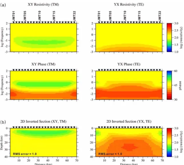
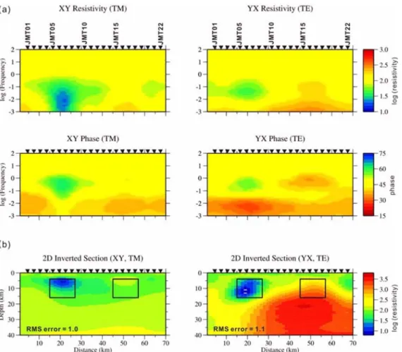
Figure 4 shows the synthetic MT responses along the profile A and 2-D inverted models of each mode obtained by the NLGC method. In TM (XY) mode, since electrical field (Ex) is parallel to the nearest coastline (i.e. northern coastline), it shows characteristics of TE mode in a regional aspect. These features can be understood from the boundary condition of electromagnetic field at the interface. That is, since the electric field parallel to the interface should be continuous across the interface, the amplitude of resulting electric field become smaller in more resistive medium. This phenomenon makes apparent resistivity lower and impedance phase higher in land- side MT responses. In contrast, the response of TE mode shows characteristics of TM mode in a regional aspect since electric field (Ey) is perpendicular to the nearest coastline. Since electrical current density

Fig. 3. (a) 1-D inverted models obtained by Occam inversion at each iteration stage for the site JMT04. (b) Observed (circle), calculated (solid line), corrected (dotted line) apparent resistivity and phase at the 3rd iteration, respectively. (c) RMS misfit between Z^o and Z at each iteration stage. The model at the initial iteration is the model without sea effect correction.

perpendicular to the interface should be continuous across the interface, hence electrical field is inevitably discontinuous at the interface and its amplitude sharply increases in more resistive medium. Due to this phenomenon, apparent resistivity become higher and phase lower in land-side MT responses. The MT responses at both the end of the profile show complex pattern due to the combined effect of the northern and western sea. Because of the these characteristics of MT responses of each mode, the inverted result for the TM responses yields conductively anomalous areas at a depth of 5-10 km and for the TE ones resistively anomalous areas below a depth of about 10km. Also,

the inverted result using both the TM and TE responses yielded a complex model combined with those of the two modes, although it was not shown in Fig. 4.

Similar to the previous section, we attempt to correct the sea effect in the 2-D responses. However, TM and TE mode respond differently to subsurface structure. In general, TE mode is especially sensitive to conductive features elongated along the strike direction, while the TM mode is sensitive to the background layered structure and also to resistive features normal to the strike (Wannamaker et al., 1989; Berdichevsky et al., 1998; Pedersen and Engels,

Fig. 4. (a) Pseudo-sections of observed MT responses for the profile A. (b) 2-D inverted models obtained by NLCG inversion for TM (XY) and TE (YX) mode prior to correcting sea effect.

Numerical Study on the Correction of Sea Effect in Magnetotelluric (MT) Data

557

2005). Therefore, it is desirable to invert using both TM and TE mode data since each mode contains complementary information about subsurface structure.

Practically, TE mode is more severely influenced by

3-D effects and often fails to reach the desired RMS error. In this case, inversion using both modes also provides unsatisfactory result. This gives us the question that which mode is more suitable to obtain a

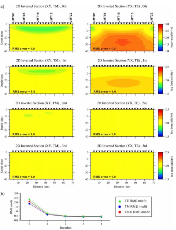
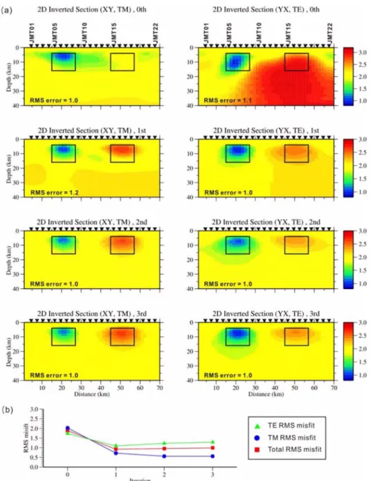
Fig. 5. (a) 2-D inverted models obtained by NLCG inversion at each iteration stage for the Model A. (b) RMS misfit between

Zo and Z at each iteration stage. Note that color palettes are re-scaled to lay stress on the differences from each iteration stage after the iteration stage 0.

reliable interpretation in 3-D environment. Berdichevsky et al. (1998) argued that both TE and TM modes should be used at various stages in the interpretation process. This is in contrast to many scientists in the western hemisphere (Wannamaker et al., 1984; Boener et al., 1999) who prefer simply to use the TM mode.

Recently, Siripunvaraporn et al. (2005) showed that fitting 3-D data with a 2-D inversion can result in spurious features, especially if TE mode data are used.

The argument above mentioned is beyond the scope of this paper, we simply utilize TM mode in order to correct the sea effect, because it is generally believed that TM mode is less influenced by 3-D effects.

We now demonstrate the sea effect correction example for synthetic data obtained along the profile A. The details for the correction step are described as follow.

(1) Add 3% random noise to

calculated from

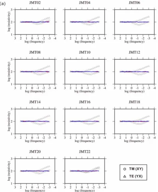
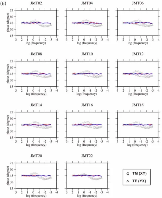
Fig. 6. (a) Apparent resistivity and (b) phase curves corresponding to Zo and Zc at the 3rd iteration stage, respectively. Triangles and circles denote the observed responses (Z^o) of each mode, while red-colored (TM) and blue-colored (TE) solid line do the corrected responses (Z^c) of each mode, respectively.

Numerical Study on the Correction of Sea Effect in Magnetotelluric (MT) Data

559

synthetic data and set it as

.

(2) Calculate

and

using 3-D forward modeling, based on 2-D inverted model of uncorrected MT response (

)

(3) Correct

and estimate

, using Eq. (3) (4) Perform 2-D inversion with TM mode data to

Zc

for a model space without the sea

(5) Calculate

and

using 3-D forward modeling, based on the 2-D model updated by the inversion to

The procedure from the step (3) to (5) is iterated until RMS misfit between

and

change become smaller than a given threshold value. Figure 5 shows the 2-D inverted model and RMS misfit at each iteration stage. The initial RMS misfit is 2.1 and it converged to 0.4 after 3 iterations. Actually, discrepancy between inverted models at the second and third iteration stage is very small. The final model is a half- space of about 102

·

, the assumed subsurface structure is closely recovered. Figure 6 shows that the

Fig. 6. Continued.

distortions due to the sea effect are successfully removed.

2-D anomalous bodies with 3-D sea (Model B) We built a 3-D model, which consists of buried 2- D anomalous bodies and 3-D sea (Model B) to test the method for a more complex 2-D structure. The

number of anomalous bodies is two: One is a conductor of 10

·

, and the other is a resistor of 1,000

·

buried in 100

·

homogeneous half- space, respectively (Fig. 7). Synthetic MT responses were generated for 24 frequencies equally spaced on a log scale between 10

and 10

Hz. All other configurations of the Model B are identical to those of

Fig. 7. 3-D model including two anomalous bodies (Model B).

Numerical Study on the Correction of Sea Effect in Magnetotelluric (MT) Data

561

the Model A, and the parameters in used 2-D NLCG inversion are also same to those of section 3.1.2.

Figure 8 shows the synthetic MT responses along the profile A and 2-D inverted models of each mode obtained by the NLGC method. In TM (XY) mode, the response of the conductor shows fairly smoothing feature and that of the resistor is hardly visible. As explained in the previous section, this is due to the decrease of the amplitude of resulting electric field (Ex). In contrast, in TE (YX) mode, the response of conductor becomes weak but clear, and that of the resistor becomes strong but spread due to the increase of the amplitude of resulting electric field (Ey). As expected, the inversion results also showed similar features. In TM mode, the imaged conductor is widely spread to horizontal direction and the resistor is

weakly imaged. In TE mode, the conductor is clearly imaged but the resistor is exaggeratedly imaged over a wide area. In addition, the inverted result using both the TM and TE responses yielded a more complex model combined with those of the two modes, although it was not shown in Fig. 8.

In parallel with the section 3.1.2, we have corrected the sea effect for the observed responses. Fig. 9 shows the 2-D inverted model and RMS misfit at each iteration stage. The initial RMS misfit is 1.9 and it converged to 0.95 after 2 iterations. The final model successfully retrieved the assumed subsurface structure after only 2 iterations. In addition, as reported by Berdichevsky et al. (1998) and Pedersen and Engels (2005), TM mode couples well to resistors while TE mode provides a better coupling to conductors.

Fig. 8. (a) Pseudo-sections of observed MT responses for the Model B. (b) 2-D inverted models obtained by NLCG inversion for TM (XY) and TE (YX) mode prior to correcting sea effect.

Conclusion

The sea effect has been an unsolved problem in land MT data in spite of a number of efforts.

Basically, this difficulty is mainly due to mutual coupling between the sea and subsurface structure. We modified the previous iterative topographic correction

method and then applied it to correct the sea effect due to surrounding seas in land MT data. Synthetic examples demonstrated that the proposed correction method closely recovers the assumed 1-D and 2-D structure of subsurface after a few iterations. This result strongly suggests that the topographic correction for seafloor MT data is greatly useful to remove

Fig. 9. (a) 2-D inverted models obtained by NLCG inversion at each iteration stage for the Model B. (b) RMS misfit between

Zo and Z at each iteration stage.

Numerical Study on the Correction of Sea Effect in Magnetotelluric (MT) Data

563 distortions due to surrounding sea in land MT data.

Finally, the proposed method can be successfully applied to real MT data which suffer from the strong sea effect and may be easily extended to 3-D structure without many efforts.

Acknowledgment

This work was supported by the Ministry of Land Transport and Maritime Affairs of Korea (grant PM 50101).

References

Baba, K. and Chave, A.D., 2005, Correction of seafloor magnetotelluric data for topographic effects during inversion. Jonrnal of Geophysical Research, 110, B12105, doi:10.1029/2004JB003463.

Baba, K.A., Chave, A.D., Evans, R.L., Hirth, G., and Mackie, R.L., 2006, Mantle dynamics beneath the East Pacific Rise at 17^oS: Insights from the Mantle Electro- magnetic and Tomography (MELT) experiment. Jonrnal of Geophysical Research, 111, B02101, doi:10.1029/

2004JB003598.

Bailey, R.C., 1977, Electromagnetic induction over the edge of a perfectly conduction ocean: The H-polariza- tion case. Geophysical Journal of Royal Astronomical Society, 48, 385-392.

Bapat, V.J., Segawa, J., Honkura, Y., and Tarits, P., 1993, Numerical estimations of the sea effect on the distribu- tion of induction arrows in the Japanese island arc.

Physics of the Earth and Planetary Interiors, 81, 215- Berdichevsky, M.N., Vanyan, L.L., and Dmitriev, V.I.,229.

1989, Methods used in the U.S.S.R to reduce near-sur- face inhomogeneity effects on deep magnetotelluric sounding. Physics of the Earth and Planetary Interiors, 53, 194-206.

Berdichevsky, M.N., Dmitriev, V.I., and Pozdnjakova, E.E., 1998, On two dimensional interpretation of magnetotel- luric soundings. Geophysical Journal International, 133, 585-606.

Berdichevsky, N.M., 1999, Marginal notes on magnetotellu- rics. Survey in Geophysics, 20, 341-375.

Boerner, D.E., Kurts, R.D., Craven, J.A., Ross, G.M., Jones, F.W., and Davis, W.J., 1999, Electrical conductiv- ity in the Precambrian lithosphere of western Canada.

Science, 283, 668-670.

Chave, A.D. and Thomson, D.J., 1989, Some comments on magnetotelluric response function estimation. Jonrnal of

Geophysical Research, 94, 14,215-14,225.

Chave, A.D. and Smith, J.T., 1994, On electric and mag- netic galvanic distortion tensor decompositions. Jonrnal of Geophysical Research, 99, 4,669-4,682.

Chave, A.D. and Thomson, D.J., 2004, Bounded Influence estimation of magnetotelluric response functions. Geo- physical Journal International, 157, 988-1,006

Constable, S.C., Parker, R.L., and Constable, C.G., 1987, Occam’s inversion: A practical algorithm for generat- ing smooth models from electromagnetic sounding data.

Geophysics, 52, 289-300.

Dosso, H.W., Chen, J., Chamalaun, F.H., and McKnight, J.D., 1996, Difference electromagnetic induction arrow responses in New Zealand. Physics of the Earth and Planetary Interiors, 97, 219-229.

Egbert, G.D. and Booker, J.R., 1986, Robust estimation of geomagnetic transfer functions. Geophysical Journal of Royal Astronomical Society, 87, 173-194.

Egbert, G.D., 1997, Robust multiple station MT data pro- cessing. Geophysical Journal International, 130, 475- Evans, R.L., Tarits, P., Chave, A.D., White, A., Heinson,496.

G., Filloux, J.H., Toh, H., Seama, N., Utada, H., Booker, J.R., and Unsworth, M.J., 1999, Asysmetric electrical structure in the mantle beneath the East Pacific Rise at 17^oS. Science, 286, 752-756.

Filloux, J.H., 1977, Ocean-floor magnetotelluric sounding over North Central Pacific. Nature, 262, 297-301.

Gamble, T.D., Goubau, W.M., and Clarke, J., 1979, Mag- netotellurics with a remote reference. Geophysics, 44, 55-68.

Groom, R.W. and Bailey, R.C., 1989, Decomposition of magnetotelluric impedance tensors in the presence of local three-dimensional galvanic distortion. Jonrnal of Geophysical Research, 94, 1,913-1,925.

Groom, R.W. and Bahr, K., 1992, Corrections for near sur- face effects: Decomposition of the magnetotelluric impedance tensor and scaling corrections for regional resistivities: A tutorial. Survey in Geophysics, 13, 341- Heison, G. and Lilley, F.E.M., 1993, An approach of thin-379.

sheet electromagnetic modeling to the Tasman Sea.

Physics of the Earth and Planetary Interiors, 81, 231- Koyama, T., 2002, A study of the electrical conductivity of251.

mantle by voltage measurements for submarine cables.

Ph.D. thesis, University of Tokyo, Tokyo.

Likelybrooks, D.W., 1986, Modeling earth resistivity struc- ture for MT data: A comparison of rotationally invari- ant and conventional earth response functions (abstact).

EOS Transactions, American Geophysical Union, 67, Mackie, R.L., Madden, T.R., and Wannamaker, P.E., 1993,918.

Three-dimensional magnetotelluric modeling using dif- ference equations-Theory and comparisons to integral equation solutions. Geophysics, 58, 215-226.

McNeice, G.W. and Jones, A.G., 2001, Multisite, multi-fre- quency tensor decomposition of magnetotelluric data.

Geophysics, 66, 158-173.

Nolasco, R.P., Smith, J.T., Filloux, J.H., and Chave, A.D., 1998, Magnetotelluric imaging of the Society Island hotspot. Jonrnal of Geophysical Research, 103, 30,287- 39,309.

Pedersen, L.B. and Engels, M., 2005, Routine 2D inver- sion of magnetotelluric data using the determinant of impedance tensor. Geophysics, 70, 33-41.

Pringle, D., Ingham, M., McKnight, D., and Chamalaun, F., 2000, Magnetovariational soundings across the South Island of New Zealand: Difference arrows and the Southern Alps conductor. Physics of the Earth and Planetary Interiors, 199, 285-298.

Rikitake, T. and Honkura, Y., 1985, Solid earth geomag- netism. Terrapub, Tokyo, 384 p.

Rodi, W.L. and Mackie, R.L., 2001, Nonlinear conjugate gradients algorithm for 2-D magnetotelluric inversion.

Geophysics, 66, 174-187.

Santos, F.A.M., Nolasco, M., Almeida, E.P., Pous, J., and Mendes-Victor, L.A., 2001, Coast effects on magnetic and magnetotelluric transfer functions and their correc- tion: Application to MT soundings carried out in SW Iberia. Earth and Planetary Science Letters, 186, 283- Shimoizumi, M., Mogi, T., Nakada, M., Yukutake, T.,295.

Handa, S., Tanaka, Y., and Uchida, H., 1997, Electrical

conductivity anomalies beneath the western sea of Kyushu, Japan. Geophysical Research Letters, 24, 1551- 1554.

Siripunvaraporn, W., Egbert, G., and Uyeshima, M., 2005, Interpretation of two-dimensional magnetotelluric pro- file data with three-dimensional inversion; Synthetic examples. Geophysical Journal International, 160, 804- Wannamaker, P.E., Hommann, G.W., and Ward, S.H., 1984,814.

Magnetotelluric responses of three-dimensional bodies in layered earths. Geophysics, 49, 1,517-1,533.

Wannamaker, P.E., Stodt, J.A., and Rijo, L., 1986, Two- dimensional topographic response in magnetotelluric modeled using finite elements. Geophysics, 51, 2,132- 2,144.

Wannamaker, P.E., Booker, J.R., Jones, A.G., Chave, A.D., Filloux, J.H., Waff, H.S., and Law, L.K., 1989, Resis- tivity cross section through the Juan de Fuca subduc- tion system and its tectonic implications. Jonrnal of Geophysical Research, 94, 14,127-14,144

Weaver, J.T. and Agarwal, A.K., 1991, Is addition of induction vectors meaningful? Physics of the Earth and Planetary Interiors, 65, 163-181.

Weaver, J.T. and Dawson, T.W., 1992, Adjustment dis- tance in TM mode electromagnetic induction. Geophysi- cal Journal International, 108, 293-300.

Yang, J.M., 2006, Automatic rejection scheme for MT and GDS data processing and interpretation on conductivity anomalies of the Korean Peninsula. Ph. D. thesis, Seoul National University, Korea, 137 p.

Manuscript received: July 31, 2008 Revised manuscript received: October 15, 2008 Manuscript accepted: October 24, 2008