Relationship between Diurnal Patterns of Transit Ridership and Land Use in the Metropolitan Seoul Area

Relationship between Diurnal Patterns of Transit Ridership and Land Use in the Metropolitan Seoul Area

Keumsook Lee* · Yena Song** · Jong Soo Park*** · William P. Anderson****

This work was supported by the National Research Foundation Grant, funded by the Korean Government (KRF-2008- 327-B00821).

* Department of Geography, Sungshin Women’s University, Seoul 136-742, Republic of Korea

** Transportation Research Group, School of Civil Engineering and the Environment, University of Southampton, Southampton, Hampshire, SO17 1BJ, U.K.

*** School of Information Technology, Sungshin Women’s University, Seoul 136-742, Republic of Korea

**** Department of Political Science, University of Windsor, Windsor, Ontario, Canada N9B 3P4

Abstract : This study investigates the time-space characteristics of intra-urban passenger flows in the Metropolitan Seoul area. In particular, we analyze the relationships between transit rider- ship and land use through the use of the subway passenger flow data obtained from the transit transaction databases. For this purpose, the strength of each subway station, i.e., the number of total in-coming and out-going passengers at each station, in the morning, afternoon, and evening, is calculated and visualized, which reflects urban land use patterns. Then the subway stations are classified into four groups via a hierarchical analysis of the in-coming and out-going passenger flows at 353 stations. Each group appears to have characteristic properties according to the region, e.g., residential areas and central business districts. This has been confirmed by the analysis which probes explicitly the relationship between the local socio-economic variables and station groups. This analysis, disclosing the inter-relationship between the subway network and urban land use, may be useful at various stages in urban as well as transportation planning, and provides analytical tools for a wide spectrum of applications ranging from impact evaluation to decision-making and planning support.

Keywords : transit transaction databases, data-mining, diurnal patterns of transit ridership,

time-space characteristics, cluster analysis, land use

1. Introduction

Intra-urban passenger flow is the outcome of urban population’s everyday life interacting with people and activities located over the urban space (Boarnet and Crane, 2001). Therefore, understand- ing the spatial textures and dynamics of urban traf- fic flows and their relations with land use variables provides fundamental insights in the realms of ur- ban and transportation planning, spatial analysis, and regional science. In particular, the interrelation between land use and intra-urban passenger traffic flow has long been of central interest to transporta- tion researchers and geographers, since intra-urban passenger flows are strongly interrelated with the spatial distribution of population and urban activi- ties as well as their functional linkages.

Many endeavors have been made for analyzing the relationships between transportation and urban land use patterns (Hansen, 1959; Alonso, 1964;

Davidson, 1977; Anas, 1982; Kim, 1983; Prastacos, 1986; Hirschman and Henderson, 1990; Guiliano, 1995; Wilson, 1998; Shaw and Xin, 2003; Geurs and Wee, 2004; Lee, et al., 2007; Chen, et al., 2009a). However, most previous studies have used passenger flow data estimated from models with surrogate variables or survey data for samples of the population. Our understanding of the time-space characteristics of urban passenger flows is thus lim- ited due to the lack of tools and data to monitor ac- tual passenger traffic flows representing entire and time-resolved movement trajectories of individuals in the urban population.

The informatics revolution has enabled system- atic gathering of passenger flow data and handling of large-scale network data sets (De Montis, et al.,

2007). By operating a smart card system, the public transportation system of Metropolitan Seoul ob- tains real passenger flow data on the real time basis.

Over 10,000,000 transaction records are stored in the large-scale passenger transaction databases per day, which contain the time-space travel trajectory information of every transit user. Recently, Park and Lee (2007, 2008) developed data mining algo- rithms for finding travel sequence paths to capture passenger travel behaviors in the transit transaction database. The problem of mining sequential pat- terns was introduced by Agrawal & Srikant (1994, 1995) as the Knowledge Discovery in Databases (KDD) for mining access patterns in environments such as World Wide Web (WWW), and extended thereafter (Park, et al., 1997; Chen, et al., 1998;

Pei, et al., 2000; Zaki, 2001). The possibility of accessing and mining large-scale data sets allows more detailed statistical analysis and theoretical characterization of correlation patterns, hierarchies, and structures of complex traffic flows (Latora and Marchiori, 2002; Chowell, et al., 2003; Sen, et al.

2003; Jiang and Claramount, 2004; Sienkiewicz and Holyst, 2005; Angeloudis and Fisk, 2006; Li, 2007; De Montis, et al., 2007; Chen, et al., 2009ab;

Lee. et al., 2008, 2011).

This paper investigates the time-space charac-

teristics of intra-urban passenger flows in the Met-

ropolitan Seoul Subway systems (MSS). Subway is

the major passenger transport mode in the Metro-

politan Seoul area, whose traffic share accounts for

more than 35% of all trips in this area. In particu-

lar, we examine strengths of subway stations, i.e.,

numbers of in-coming and out-going passengers,

and their relation with land use variables. For that

purpose, we analyze the inflow/outflow data of 353

subway stations in the MSS for three time zones of

a day (morning, afternoon, evening), obtained by a data mining algorithm developed by Park and Lee (2007, 2008). The spatial patterns and structures of passenger flows are analyzed by means of a cluster analysis technique which allows us to classify the subway station groups according to the passenger flow patterns over the three time zones. Then the relationship between the subway passenger flow pattern and the local economic structures is investi- gated, which reveals the interactions between pub- lic transport passenger flows and land use patterns.

2. Study Area and Data

Metropolitan Seoul (see Figure 1) is the most

densely populated and developed area in Korea, ac- commodating approximately 23,000,000 inhabit- ants in the area 12,446 km

. It accounts for 48.4%

of the total national population and 11.8% of the total national area. This area has long suffered from severe traffic congestion. Since many urban activi- ties are concentrated in this region (68% of total national financial transactions, 95% of entrepre- neur headquarters, 57% of manufacturing firms, 40% of colleges/universities, and 85% of public ad- ministration offices), large volumes of traffic flows are generated. Rail transit supplemented by con- necting bus systems is the most popular transporta- tion mode for passenger movements, accounting for two-thirds of the total passenger traffic flows in this area. A unified fare structure is in effect, treat- ing the whole public transport network as a single

Figure 1. Study Area: Metropolitan Seoul in Korea

mode with charges being applied to transaction units.

The “smart card” system based on integrated circuit cards (ICCs) has been adopted in the public transportation system in Metropolitan Seoul and is used by more than 90% transit users. In addition to the travel efficiency benefits of this system, it also allows collection of transit users’ travel trajec- tory data in the Metropolitan Seoul area. Since each passenger’s transit fare is determined for a trip chain from the first boarding to the last alighting, each card user’s movement is tracked by the Global Positioning System (GPS) for keeping the locations and times of departures, transfers, and destina- tions, and stored in the transit transaction databas- es. On a normal weekday, over 10,000,000 transac- tions have been stored in the smart-card transaction databases in Metropolitan Seoul since July 1, 2004 and that number has been doubled since July 1, 2007 when the smart card system was extended to the bus system outside the central city.

The system makes it possible to track the move- ments of individuals, for the transit transaction database contains time/space information of each passenger’s travel and each smart card has its own identification (ID). Passenger flows can be com- puted based on the travel sequence path of each passenger mined from the large-scale transit trans-

action database with the help of the data mining algorithms (Park and Lee, 2007, 2008). In this pa- per we use the single-day-transit transaction data- base on June 24, 2005, which contains 10,667,519 transactions with the information on 24 trip- related attributes for each transaction, and focus only on subway passenger flows excluding transac- tions occurred solely on buses. This leaves us with 4,907,541 transactions of subway passengers, giving the information about the time/location of get-on/- off.

As majorities of passengers have different travel purposes depending on the time zone of a day, the spatial distribution patterns of passenger flows vary over the time zone. For simplicity, we divide a day into three time zones: morning (before 11 am), afternoon (11 am to 5 pm), and evening (after 5 pm), to catch the time-space characteristics of intra- urban passenger flows. By recording information on get-on/off of each transit user in the get-on/off matrix, we obtain the passenger flows and summa- rize in Table 1 the total passenger flows in each time zone and between time zones.

We adopt a weighted network representation in such a way that nodes correspond to subway sta- tions and links to actual passenger flows between subway stations in the MSS, which consists of eight subway lines and N=353 stations. The weighted Table 1. Passenger Distribution by Time Zones

Get-off

Get-on Morning Afternoon Evening Total

Morning 1,585,358 86,510 23 1,671,891

Afternoon 0 995,686 132,796 1,128,482

Evening 0 0 2,107,168 2,107,168

Total 1,585,358 1,082,196 2,239,987 4,907,541

graph representation allows one to consider fea- tures pertaining to the traffic flows on networks (De Montis, et al, 2007). We thus construct the weighted passenger flow matrix W, the element w

of which corresponds to the passenger flow from station i to station j based on the location/time in- formation from each passenger’s transaction record.

Namely, the weight of a link between a pair of sta- tions in each time zone is obtained by counting the passengers between them within the time period.

Note that the weight w

represents the directed pas- senger flow on the link from i to j, and we thus have N (N - 1) passenger flows in each time zone.

3. Spatial Structure of Intra Urban Passenger Flows

Recently, statistical and dynamic characteristics of network structures and passenger flows in the MSS have been analyzed (Lee, et al., 2008, 2010, 2011). The strength of each station describing the number of total incoming and outgoing passengers at the station as well as the weight between a pair of stations in a day has been examined.

In this study, we consider separately the inflow strength and the outflow strength of each station, corresponding respectively to the number of in- coming passengers and that of outgoing passengers, in each of the three time zones. We then analyze their relations to land use variables, which disclose the time-space characteristics of passenger flows in the MSS.

The inflow I

and the outflow O

of station i are defined to be

I

≡ ∑

j=1

w

(1)

and

O

≡

∑

w

(2)

respectively, where the weight wij again repre- sents the number of passengers traveled from i to j and N is the total number of stations. Accordingly, the (total) strength of station i is given by

S

≡I

+O

=

^∑

(w

+w

) (3)

In order to investigate spatial variations in the flows over the three time zones, we visualize the spatial patterns and structures of inflows/outflows by means of the inverse distance technique. As shown in Figure 2a, inflows are concentrated at the central business districts (CBDs) in the southeast- ern center and in the northern center and at a few sub-CBDs while the outflows are distributed heav- ily in the large residential areas located over the out- skirts of Seoul City in the morning (see Figure 2f).

In the afternoon, the passenger flows become some- what weakened, although their distributions are still concentrated at the CBDs and sub-CBDs, the southeastern CBD in particular (see Figures 2b and 2e). Since people are staying at the CBDs and sub- CBDs, these areas discharge heavy outflows in the evening (see Figure 2d). On the other hand, inflows are distributed not only at the residential areas but also at various activity centers, including business, entertainment, social, and commercial districts (see Figure 2c). This manifests that people tend to visit several places rather than to go back home directly after work at the CBD area (Lee, et al., 2010).

Figure 2 manifests that stations in different

locations may serve different purposes and some may share similar patterns. To probe the subway travel pattern and its relation with socio-economic factors, we employ the cluster analysis to group stations according to passenger flow patterns and explore socio-economic properties of each station group.

The variables used in the cluster analysis are the numbers of departures/arrivals at stations. As in the previous study by Lee, et al. (2007), subway trips are differentiated according to the travel time zone (morning, afternoon, and evening) as well as to whether they correspond to the inflow or outflow of passengers; this leads to six variables for each

station. To describe similarity and dissimilarity, we measure distances among individuals through the use of Ward’s minimum variance clustering method (Ward, 1963). To decide the optimal num- ber of clusters, we employ four statistics: average silhouette, Herbert’s gamma, Dunn’s index, and the withindistance/ between distance ratio. The statistics indicates that three or four clusters would be reasonable and it is concluded that four clusters would be the best.

Properties of each group in the four-cluster mod- el are shown in Table 2. Such quantities as the di- ameter

, average distance

, and median distance

describe the dissimilarity within a cluster: The big- Figure 2. Spatial Patterns of Passenger Flows

(a) (b) (c)

(d) (e)

(f)

ger they are, the less similar the observations within a cluster are. On the other hand, the separation

and average distance to others

are related with the distance from one cluster to another. Finally, the average silhouette is calculated by considering both of within and between clusters’ dissimilarity.

The most distinctive group is the first one: It is most separated from others according to the separa- tion measure and average distance to others. Inter- estingly, most of the stations in Group 1 are located in Seoul CBDs, sub-CBDs, or other city centers.

Stations in Group 2 surround those in Group 1 sta- tions and are mostly located near Seoul CBDs with a few exceptions in city centers in southern Seoul.

Group 3, including almost two-thirds of all the stations, exhibits most similarity within the group as well as the least separation from others. Finally,

Group 4 consists mainly of stations located out of CBD regions or big city centers.

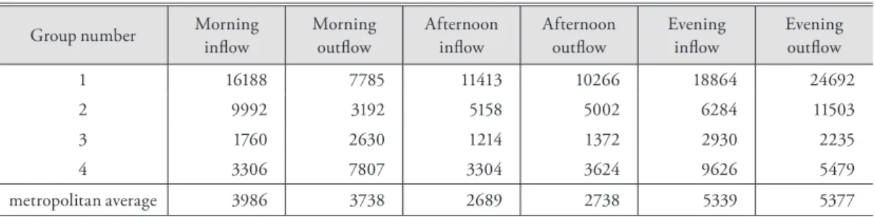
Table 3 shows the average inflow and outflow in each group. In general, stations in Group 1 are the busiest with highest usages all over the time zones, and those in Group 3 are the least used. It is natu- ral that working places would show high morning arrivals and residential areas high morning depar- tures, and vice versa in the evening flows. From this point of view, Groups 1 and 2, having relatively high morning inflows, are expected to include those stations located at working places. On the contrary, Groups 3 and 4 show relatively large values of out- flow in the morning and of inflow in the evening, implying stations in residential areas.

It is of interest to observe that afternoon inflow and outflow are almost the same in all groups. One Table 2. Statistical Properties of the Four Groups

Group Number 1 2 3 4

Size 25 54 239 46

Diameter 57462 23460 11537 13973

Average distance 21295 8960 3774 5456

Median distance 18267 7834 3532 4814

Separation 4957 1487 997 997

Average distance to others 34126 15279 17649 12092

Average silhouette 0.115 0.193 0.606 0.396

Table 3. Average Inflow and Outflow in Each Group Group number Morning

inflow Morning

outflow Afternoon

inflow Afternoon

outflow Evening

inflow Evening outflow

1 16188 7785 11413 10266 18864 24692

2 9992 3192 5158 5002 6284 11503

3 1760 2630 1214 1372 2930 2235

4 3306 7807 3304 3624 9626 5479

metropolitan average 3986 3738 2689 2738 5339 5377

possible explanation stems from the difference in the trip purpose depending on the time zone: The purpose of a trip in the afternoon is mostly some-

thing other than commuting, e.g., business, shop- ping, and personal affairs. Such activities usually do not require staying for a long time and round trips

Table 4. Population Characteristics by Groups

Population Characteristics 1 2 3 4 metropolitan average ANOVA (F value)

Average population 17458 15828 23526 22216 21988 1.185

Sex ratio 100.04 103.65 110.27 98.66 107.23 0.159

Working population ratio 80.16 77.67 75.32 76.47 76.10 23.617**

Average population density 15.87 13.63 19.60 28.67 19.79 13.303**

Median age 34.58 35.76 34.40 33.89 34.51 4.299**

** 99% significance, * 95% significance

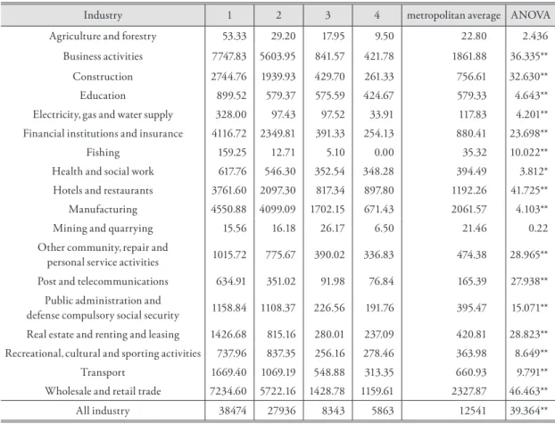
Table 5. Industrial Characteristics by Groups

Industry 1 2 3 4 metropolitan average ANOVA

Agriculture and forestry 53.33 29.20 17.95 9.50 22.80 2.436

Business activities 7747.83 5603.95 841.57 421.78 1861.88 36.335**

Construction 2744.76 1939.93 429.70 261.33 756.61 32.630**

Education 899.52 579.37 575.59 424.67 579.33 4.643**

Electricity, gas and water supply 328.00 97.43 97.52 33.91 117.83 4.201**

Financial institutions and insurance 4116.72 2349.81 391.33 254.13 880.41 23.698**

Fishing 159.25 12.71 5.10 0.00 35.32 10.022**

Health and social work 617.76 546.30 352.54 348.28 394.49 3.812*

Hotels and restaurants 3761.60 2097.30 817.34 897.80 1192.26 41.725**

Manufacturing 4550.88 4099.09 1702.15 671.43 2061.57 4.103**

Mining and quarrying 15.56 16.18 26.17 6.50 21.46 0.22

Other community, repair and

personal service activities 1015.72 775.67 390.02 336.83 474.38 28.965**

Post and telecommunications 634.91 351.02 91.98 76.84 165.39 27.938**

Public administration and

defense compulsory social security 1158.84 1108.37 226.56 191.76 395.47 15.071**

Real estate and renting and leasing 1426.68 815.16 280.01 237.09 420.81 28.823**

Recreational, cultural and sporting activities 737.96 837.35 256.16 278.46 363.98 8.649**

Transport 1669.40 1069.19 548.88 313.35 660.93 9.791**

Wholesale and retail trade 7234.60 5722.16 1428.78 1159.61 2327.87 46.463**

All industry 38474 27936 8343 5863 12541 39.364**

Average industrial employment by industry and groups

** 99% significance, * 95% significance

are completed within the same time zone, contrib- uting to afternoon flows.

4. Passenger Flows and Land Use

Travel patterns are related closely to land-use characteristics (Kitamura, et al., 1998; Boarnet and Crane, 2001). For example, if retail shops are highly concentrated at a certain part of a city, a significant level of shopping trips would be generated to and from that area. Similarly, residential areas would show high levels of departure trips in the morning and of arrival trips in the evening due to the travel demand for commuting. In short, passenger flows may be expressed as a function of land-use charac-

teristics.

In our case, the difference between inflow and

outflow along with the cluster location map dis-

closes that the stations in Groups 1 and 2 are likely

to be in working places and those in Groups 3 and

4 in residential areas. To confirm the inference

from inflow and outflow patterns, we also overlay

land-use variables of the places where stations be-

longing to each group are located. Tables 4 and 5

show population and employment characteristics of

each group such as number of residents, industrial

employment levels, respectively. From the tables

in Tables 4 and 5, it is observed that the total em-

ployment level in Group 1 is three times above the

average. Group 2 also shows a high employment

level while others have below the average numbers

of employees. This manifests spatial characteristics

Figure 3. Employment Shares by Groups

of the stations in Groups 1 and 2, which are in fact expected from the previous statistics.

It is also interesting to examine the industrial mix ratio among groups, displayed in Figure 3.

Although Metropolitan Seoul is densely developed and clustering has been obtained from the flow characteristics of stations, each group has a distinc- tive mixture of industries. The locations of Group 1, mainly CBDs and city centers, correspond to more of the knowledge-intensive service region, oriented toward business activities and financial in- dustries. Group 3 is dominated by the manufactur- ing industry and Group 2 by sales and business ac- tivities. Finally, Group 4 is characterized by its least share of the knowledge sector and relatively high proportion of hotel and restaurant employment.

In investigating the relation between passenger

flows and land-use variables, it would be desirable to consider strength variations over time and differ- ence between inflow and outflow, instead of adopt- ing the total strength of each station for a day. In this sense, multinomial logit (MNL) is applied to station groups established from the cluster analysis in the previous section. In our model, the depen- dent variable is the cluster group, and these groups do not have any order nor is one group nested to another. Thus basic MNL is applied and model is defined as:

P(y

= j)=

1+

^∑

exp(X

β

) exp(X

β

)

(4)

where P(y

= j) denotes the probability that the de- pendent variable y takes the value of j (= 1, 2, 3, and Table 6. Model Summary

Variables

Group 1 over Group 3 Group 2 over Group 3 Group 4 over Group 3 Coefficient Standard

Error Coefficient Standard

Error Coefficient Standard Error

Constant - 48.809** 8.121 - 24.727** 6.241 -8.847 5.347

Population Density 0.025 0.030 - 0.015 0.025 0.048** 0.015

Working

Population (R) 0.331** 0.090 0.136 0.070 0.065 0.066

(log) Total

Employment 1.677** 0.506 1.159** 0.318 0.121 0.318

Business

Activities (R) 0.064 0.042 0.073** 0.027 - 0.039 0.036

Education (R) 0.096** 0.037 - 0.011 0.046 - 0.043 0.032

Finance (R) 0.099* 0.045 0.003 0.039 0.021 0.042

Hotel and

Restaurant (R) 0.101* 0.052 0.016 0.045 0.074* 0.029

Sales (R) 0.081** 0.030 0.057** 0.021 - 0.018 0.027

Summary Stats. Number of

observations 353 Log

likelihood - 245.95 Residual

deviance 491.906 on 1032 D.F.

* indicates significance at the 95% level; ** 99% of significance.

(R) stands for the ratio.

4) at the ith observation, X

is a vector of indepen- dent variables, and β

’s are unknown parameters.

The MNL model is estimated by means of the maximum likelihood method, with Group 3 cho- sen as the comparison category. Namely, the prob- ability of being classified as Group 1, 2, or 4 is com- pared with the probability of membership in the reference category. Group 3 is selected as the refer- ence since it contains over 2/3 of the stations in the MSS, thus shows the most common passenger flow pattern. Among a number of possible combinations of independent variables which lead to different models, the best model is selected on the basis of the Akaike Information Criterion (AIC) and the Bayesian Information Criterion (BIC).

The coefficient estimated for cluster memberships are given in Table 6. One consensus from resultant coefficients is that significant coefficients appear to be positive except constants; this implies that if a station is located where any of independent vari- ables have significantly high values, it is likely to be classified as Group 1, 2, or 4. Specifically, more working population proportions, higher total em- ployment levels, and high employment ratios of fi-

nance, education, hospitality, and sales sectors lead corresponding stations more probable to be classi- fied as Group 1 against Group 3. The chance to be a member of Group 2 compared with that of Group 3 increases as the station is located in the area with high levels of employment, business activities, and sales. Finally, stations in densely population regions or high levels of hotel and restaurant employment are inclined to belong to Group 4 instead of Group 3.

It should be noted that the coefficients of the MNL model do not be interpreted as the ones from regression models since they do not represent marginal effects of the independent variables. For instance, the coefficients of Group 1 only imply the effects that the independent variables have on prob- ability of being Group 1 relative to the reference, Group 3. However, taking the derivative of the MNL equation above, we obtain a marginal effect measurement as below (Greene, 2003):

δ

= ∂P

∂X

=P

( ^β

^-

^∑

^P

^β

) ^≡P

^{( β}

^{- β - ) (5)}

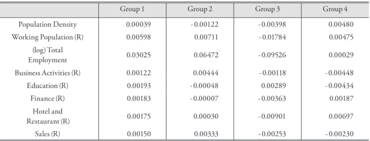
Table 7 shows the marginal effects of each inde-

Table 7. Marginal Effects

Group 1 Group 2 Group 3 Group 4

Population Density 0.00039 - 0.00122 - 0.00398 0.00480

Working Population (R) 0.00598 0.00711 - 0.01784 0.00475

(log) Total

Employment 0.03025 0.06472 - 0.09526 0.00029

Business Activities (R) 0.00122 0.00444 - 0.00118 - 0.00448

Education (R) 0.00193 - 0.00048 0.00289 - 0.00434

Finance (R) 0.00183 - 0.00007 - 0.00363 0.00187

Hotel and

Restaurant (R) 0.00175 0.00030 - 0.00901 0.00697

Sales (R) 0.00150 0.00333 - 0.00253 - 0.00230

pendent variable on being a member of each group, which describes changes in the probability to be a member of a certain group under the condition of 1% increase of each independent variable whilst other variables remain at the mean value. Although the marginal changes are not big in most cases, there is a noticeable contrast between Groups 1 and 3: While Group 1 has all positive, in Group 3 all but education employment share are negative.

In particular, 1% increase in the total employment (logged) would decrease the chance being in Group 3 by almost 10%, which is the biggest effect of the change of a single variable. Such opposite charac- teristics in the population and employment pat- tern support our previous findings from passenger inflow and outflow data by groups. Namely, Group 1 stations are in CBDs and city centers whereas Group 3 mostly in residential areas.

5. Conclusion

This work has investigated the time-space char- acteristics of intra-urban passenger flows in the Metropolitan Seoul area in which subway system transports a majority of passenger trips. In particu- lar, we have probed cluster structures of passenger flows in three time zones of a day (morning-, after- noon-, and evening-time) and their relations to the travel time and land-use variables. For this purpose, we have analyzed actual passenger flows mined from one-day-transit transaction databases which contain each passenger’s travel trajectory data for all the transit users in Metropolitan Seoul.

The results of our analysis may be useful at vari- ous stages in urban planning as well as transporta-

tion planning, and provide analytical tools for a wide spectrum of applications ranging from impact evaluation to decision-making and planning sup- port. Understanding travel patterns in a metropoli- tan area is a big task that must be achieved for an ef- ficient planning process. The information provided in this study is especially useful for public transpor- tation and regional planning: We have utilized real travel data, which are reported not by individuals but by travel card records, thus provide precise and objective numbers as to subway travel patterns. This is in contrast with existing studies, which, due to the unavailability and/or restrictions of objective travel data, used self-reported data, mostly from survey questionnaires from sampled population.

Unlike those precedents, up-to-date technology has allowed us to access and analyze the objective travel data set storing more than 90% of all trips made in a given day.

Finally, note that data of only one day of a year

have been analyzed here. In general, changes in the

existing network can alter travel behaviors and land

use development patterns as well as network acces-

sibility. While smart card data have existed since

2004, one more subway line was launched in 2009

as well as several extension links were added. Al-

though it may not be feasible to go back to an early

stage of the subway network in Metropolitan Seoul,

and to examine travel patterns as in this study, we

can trace changes in the travel behavior due to the

addition of infrastructure when a stable data set is

available for the year of 2009 or later. Further, with

the help of explorative data analysis tools, residen-

tial and working areas are identifiable. In the future

study, more accurate and sophisticated analysis is

expected to be performed with more variables and

refined methodologies, relating individual travel

behaviors to land use development patterns.

Notes

1) For mapping the strength of each point (i.e., station) in the raster form, the inverse distance techinque has been ad- opted.

2) maximum within cluster distance 3) within cluster average distance 4) within cluster median distance

5) cluster-wise minimum distance between a point in the clus- ter and a point in other cluster

6) cluster-wise average distance between a point in the cluster and a point in other cluster

References

Agrawal, R. and Srikant, R., 1994, “Fast algorithms for mining association rules in large databases,” Pro- ceedings of the 20th International Conference on Very Large Databases, 478-499.

Agrawal, R. and Srikant, R., 1995, “Mining sequential pat- terns,” Proceedings of the 11th nternational Confer- ence on Data Engineering, 3-14.

Alonso, W., 1964, Location and Land Use, Harvard Uni- versity Press: Cambridge, M.A.

Anas, A., 1982, “Residential Location Models and Urban Transportation,” Economic Theory, Econometrics, and Policy Analysis with Discrete Choice Models, Academic Press: New York.

Angeloudis, P. and Fisk, D., 2006, “Large subway systems as complex networks,” Physica A 367, 553-558.

Boarnet, M. and Crane, R., 2001, “The influence of land use on travel behavior: specification and estima- tion strategies,” Transportation Research Part A 35, 823-845.

Chen, C., Chen, J. and Barry, J., 2009a, “Diurnal pattern

of transit ridership: a case study of the New York City subway system,” Journal of Transport Geogra- phy 17, 176-186.

Chen, F., Wu, Q., Zhang, H., Li, S. and Zhao, L., 2009b,

“Relationship analysis on station capacity and passenger flow: a case of Beijing subway line 1,”

Journal of Transportation Systems Engineering and Information Technology 9(2), 93-99.

Chen, M. S., Park, J. S., and Yu, P. S., 1998, “Efficient data mining for path traversal patterns,” IEEE Transac- tions on Knowledge and Data Engineering 10(2), 209-221.

Chowell, G., Hyman, J. M., Eubank, S., and Castillo- Chavez, C., 2003, “Scaling laws for the movement of people between locations in a large city,” Physi- cal Review E 68, 066102.

Davidson, K. B., 1977, “Accessibility in transport/land use modeling and assessment,” Environment and Plan- ning A 5, 1401-1416.

De Montis, A., Barthelemy, M., Chessa, A., and Vespig- nani, A., 2007, “The structure of interurban traf- fic: a weighted network analysis,” Environment and Planning B: Planning and Design 34(5), 905- 924. 

Geurs K. T., and B. Wee, 2004, “Accessibility evaluation of land-use and transport strategies: review and re- search directions”, Journal of Transport Geography 12: 127-140.

Giuliano, G., 1995, “Land use impacts of transportation investments: highway and transit,” in Hansen, S. (Ed.) The Geography of Urban Transportation, Guilford Press: New York, 305-341.

Greene, W .H., 2003, Econometric Analysis, Prentice Hal:

New Jersey.

Kim, T. J., 1983, “A combined land use-transportation model when zonal travel demand is endogenously determined,” Transportation Research 17B, 449- 462.

Kitamura, R., Chen, C., Narayanan, R., 1998. Traveler,

destination choice behavior: effects of time of day,

activity duration, and home location. Transporta- tion Research Record 1645, 76-81.

Hansen, W.G., 1959, “How Accessibility Shapes Land Use,” Journal of the American Institute of Planners 25, 73-76.

Hirschman, I. and Henderson, M., 1990, “Methodology for accessing local land use impacts of highways,”

Transportation Research Record 1274, 35-40.

Jiang, B., and Claramount, C., 2004, “Topological analy- sis of urban street networks,” Environment and Planning B: Planning and Design 31, 151-162.

Latora, V. and Marchiori, M., 2002, “Is the Boston subway a small-world network?,” Physica A 314, 109-113.

Lee, K., Hong, J., Min, H., and Park, J. S., 2007, “Rela- tionships between topological structures of traf- fic flows on the subway networks and land use patterns in the metropolitan Seoul,” Journal of Economic Geographical Society of Korea 10(4), 427- 443.

Lee, K., Jung, W. S., Park, J. S., and Choi, M. Y., 2008,

“Statistical analysis of the metropolitan Seoul subway system: network structure and passenger flows,” Physica A 387, 6231-6234.

Lee, K., Park, J.S., Choi, H., Choi, M.Y., and Jung, W.-S., 2010, “Sleepless in Seoul: ‘The ant and the me- trohopper,” Journal of the Korean Physical Society 57(4), 823-825.

Lee, K., Goh, S., Park, J. S., Jung, W.-S., and Choi, M.

Y., 2011, “Master equation approach to the intra- urban passenger flow and application to the Met- ropolitan Seoul Subway system,” Journal of Physics A: Mathematical and Theoretical, 44, stacks.iop.

org/JPhysA/115007.

Li, Y., 2007, “Static and dynamic complexity analysis of urban public transportation network: a case in Shanghai,” IEEE 1-4244-1312, 6376-6379.

Park, J. S., Chen, M.-S., and Yu, P. S., 1997, “Using a hash- based method with transaction trimming for mining association rules,” IEEE Transactions on Knowledge and Data Engineering 9(5), 813-825.

Park, J. S. and Lee, K., 2007, “Mining trip patterns in the large trip-transaction database and analysis of travel behavior,” Journal of the Economic Geograph- ical Society of Korea 10(1), 44-63.

Park, J. S. and Lee, K., 2008, “Network structures of the metropolitan Seoul subway systems,” Journal of the Economic Geographical Society of Korea 11(3), 459-475.

Pei, J., Han, J., Mortazavi-Asl, B., and Zhu, H., 2000,

“Mining access patterns efficiently from web logs (PDF),’ Proceedings of 2000 Pacific-Asia Conference on Knowledge Discovery and Data Mining.

Prastacos, P., 1986, “An integrated land use-transportation model for the San Francisco region: 1. Design and mathematical structure,” Environment and Plan- ning 18A, 307-322.

Sen, P., Dasgupta, S., Chatterjee, A., Sreeram, P. A., Mukherjee, G., and Manna, S. S., 2003, “Small world properties of the Indian railway network,”

Physical Review E 67, 036106.

Shaw, S. L., Xin, X., 2003, “Integrated land use and trans- portation interaction: a temporal GIS exploratory data analysis approach,” Journal of Transport Geog- raphy 11, 103-115.

Sienkiewicz, J. and Holyst, J. A., 2005, “Statistical analysis of 22 public transport networks in Poland,” Physi- cal Reviews E 72, 046127.

Ward, J. H., 1963, “Hierarchical grouping to optimize an objective function,” Journal of the American Statis- tical Association 58 (301), 236-244.

Wilson, A.G., 1998, “Land-use/transport interaction mod- els. Past and future,” Journal of Transport Econom- ics and Policy 32, 3-26.

Zaki, Mohammed J., 2001, “SPADE: an efficient algo- rithm for mining frequent sequences,” Machine Learning 42(1/2), 31-60.

Correspondence: Keumsook Lee, 249-1 Dongseon-dong 3-ga, Seongbuk-gu, Seoul 136-742, Korea, Tel:

02)920-7138, E-mail: [email protected]

교신: 이금숙, 136-742, 서울특별시 성북구 동선동 3가 249-1, 성신여자대학교 지리학과, 전화: 02-920- 7138, e-mail: [email protected]

최초투고일 2012년 2월 10일

최종접수일 2012년 2월 28일

서울 대도시권 하루 시간대별 지하철 통행흐름 패턴과 토지이용과의 관계

이금숙*·송예나**·박종수***·William P. Anderson****

요약 : 본 연구에서는 서울 대도시권에서 도시 내 통행흐름의 시-공간적 특성을 밝히고자 한다. 특히, 서울대도시권 대중교통이용자의

통행기록을 담고 있는 교통카드 데이터베이스에서 지하철 이용자의 하루 동안의 탑승자료를 이용하여 시간대별 통행흐름의 유형과 토 지이용과의 관계를 분석하였다. 이를 위하여 먼저 각 지하철역별 아침, 낮, 저녁 시간대별 승하차 여객 수를 산출하고, 그의 공간적 분포 를 GIS를 이용하여 시각화 하였다. 이러한 각 역의 시간대별 승객의 타고 내리는 승객흐름을 바탕으로 계층적 군집분석법을 이용하여 서울대도시권 지하철체계를 구성하고 있는 353개 역들을 유형화 하였다. 이러한 승객 흐름의 유형별 군집에 따라 지하철 역 인접 지역 의 토지이용을 나타내는 지역변수들과의 관계식을 도출하였다. 이러한 분석의 결과는 교통계획은 물론 도시계획의 다양한 단계에 유용 하게 이용될 수 있다.

주요어 : 교통카드 데이터베이스, 데이터마이닝, 하루 시간대별 통행흐름, 시공간적 특징, 군집분석, 토지이용 한국경제지리학회지 제15권 제1호 2012(26~41)

* 성신여자대학교 지리학과 교수

** 영국 University of Southampton, Transportation Research Group 연구원

*** 성신여자대학교 IT학부 교수

**** 캐나다 University of Windsor, Department of Political Science 교수