Prediction of Daily Patient Numbers for a Regional Emergency Medical Center using Time Series Analysis

(1)

I. Introduction

In recent years, supply has failed to keep up with continu- ous increases in the demand for emergency medical services [1], which has resulted in problems with overcrowding in Emergency Departments (ED) [2-4]. ED overcrowding has been shown to affect not only patient satisfaction, but also the quality of treatment and prognosis [5-8]. A variety of measures have been taken thus far to address this ED crowding problem [9-11], including staff supplementation, expansions of beds and spaces, diversification of test equip- ment, the establishment of walk-in clinics for the treatment of light illnesses, hallways, operation of observation units, and allocations of staff and resources according to demand [12,13]. Several studies concerning demand forecasting for allocation of staff and resources have been already been conducted [14-16]. In the emergency medical services field, Spencer et al. previously attempted to forecast demand in the ED using a variety of time series analysis methods [17],

Prediction of Daily Patient Numbers for a Regional Emergency Medical Center using Time Series Analysis

Hye Jin Kam, MS*, Jin Ok Sung, MS*, Rae Woong Park, MD, PhD

Department of Biomedical Informatics, School of Medicine, Ajou University, Suwon, Korea

Objectives: To develop and evaluate time series models to predict the daily number of patients visiting the Emergency Department (ED) of a Korean hospital. Methods: Data were collected from the hospital information system database. In order to develop a forecasting model, we used, 2 years of data from January 2007 to December 2008 data for the following 3 consecutive months were processed for validation. To establish a Forecasting Model, calendar and weather variables were utilized. Three forecasting models were established: 1) average; 2) univariate seasonal auto-regressive integrated moving average (SARIMA); and 3) multivariate SARIMA. To evaluate goodness-of-fit, residual analysis, Akaike information criterion and Bayesian information criterion were compared. The forecast accuracy for each model was evaluated via mean absolute percentage error (MAPE). Results: The multivariate SARIMA model was the most appropriate for forecasting the daily number of patients visiting the ED. Because it’s MAPE was 7.4%, this was the smallest among the models, and for this reason was selected as the final model. Conclusions: This study applied explanatory variables to a multivariate SARIMA model. The multivariate SARIMA model exhibits relativelyhigh reliability and forecasting accuracy. The weather variables play a part in predicting daily ED patient volume.

Keywords: Emergency Medical Service, Crowding, Trends, Seasonal Variation, Statistical Models

Healthc Inform Res. 2010 September;16(3):158-165.

doi: 10.4258/hir.2010.16.3.158 pISSN 2093-3681 • eISSN 2093-369X

Received for review: May 7, 2010

Accepted for publication: September 9, 2010 Corresponding Author

Rae Woong Park, MD, PhD

Department of Biomedical Informatics, School of Medicine, Ajou University, San 5, Woncheon-dong, Yeongtong-gu, Suwon 443- 721, Korea. Tel: +82-31-219-5342, Fax: +82-31-219-4471, E-mail:

veritas@ajou.ac.kr

*These authors contributed equally.

This article is based on a thesis submitted in partial fulfillment of the Mas- ter of Science degree, Ajou University School of Medicine.

This is an Open Access article distributed under the terms of the Creative Com- mons Attribution Non-Commercial License (http://creativecommons.org/licenses/by- nc/3.0/) which permits unrestricted non-commercial use, distribution, and reproduc- tion in any medium, provided the original work is properly cited.

(2)

and Sun et al. [18]. forecasted the numbers of daily patients in individual ED by considering multivariate factors. Lee et al. [19] employed multiple linear regressions to analyze the factors affecting the number of patients visiting ED in Korea.

However, thus far, no studies have been conducted regarding forecasts of the daily numbers of patients visiting ED.

The principal objective of this study was to construct a mo del by which the number of patients visiting a regional emergency center per day could be predicted, considering calendar and weather data using a moving average, univariate seasonal auto-regressive integrated moving average (SARIMA) and multivariate SARIMA; these models were compared and evaluated.

II. Methods

1. Data Sources

This study was conducted according to a retrospective study design that utilizes a dataset extracted from a tertiary hospital information system (HIS) database. The data utilized for analysis include 189,511 events involving patients who visited the ED from January 2007 to March 2009, excluding their identities (names and hospital numbers). The data for the first two years (Jan. 2007 to Dec. 2008) were used to construct the demand forecast model, whereas those from the past three months (Jan. to Mar. 2009) were used to evaluate the model. Weather data were acquired from the weather

agency’s website [20].

2. Ethical Consideration

This study employed the summed numbers of patients visiting the ED per day, and utilized no identifications or patients’ personal information. Therefore, this study was not subject to review by the Institutional Review Board.

3. Data Preprocessing and Variable Selection

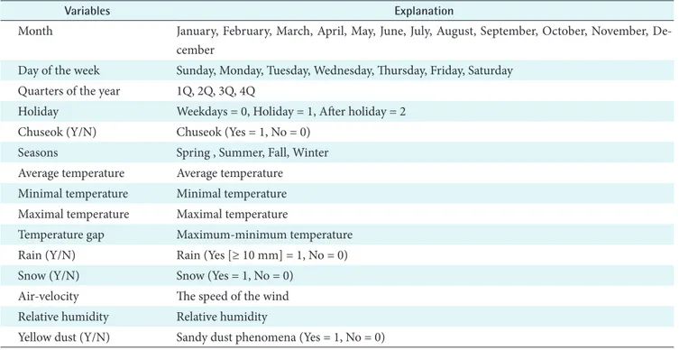
The daily number of patients visiting the ED was employed as a dependent variable, whereas information including the month, day of the week, quarter of the year, holidays, Chuseok [Y/N], seasons, weather factors [20] (average temperature, minimal temperature, maximal temperature, temperature gap, rain [Y/N], snow [Y/N], air-velocity, relative humidity, and yellow dust [Y/N]) were employed as independent variables (Table 1).

The number of patients visiting the ED per day was calculated by counting the number of visiting patients from midnight to the following midnight. Holidays include public holidays and Sundays. Weekdays immediately following a holiday and Saturdays are defined as “After Holiday”.

Chuseok, which differs significantly from other holidays, is classed as a separate variable. Quantities of precipitation exceeding 10 mm, which ordinary people tend to regard as a significant amount of rain, was the threshold for raining”.

The operational definition for “snowing” in this study was as

Table 1. Definition of variables

Variables Explanation

Month January, February, March, April, May, June, July, August, September, October, November, De- cember

Day of the week Sunday, Monday, Tuesday, Wednesday, Thursday, Friday, Saturday Quarters of the year 1Q, 2Q, 3Q, 4Q

Holiday Weekdays = 0, Holiday = 1, After holiday = 2 Chuseok (Y/N) Chuseok (Yes = 1, No = 0)

Seasons Spring , Summer, Fall, Winter Average temperature Average temperature Minimal temperature Minimal temperature Maximal temperature Maximal temperature

Temperature gap Maximum-minimum temperature Rain (Y/N) Rain (Yes [≥ 10 mm] = 1, No = 0) Snow (Y/N) Snow (Yes = 1, No = 0)

Air-velocity The speed of the wind Relative humidity Relative humidity

Yellow dust (Y/N) Sandy dust phenomena (Yes = 1, No = 0)

(3)

abundance of piled-up snow, which again exceeds the gen- eral notion of “snowing”.

4. Modeling Technique

For this study, the moving average method, the univariate SARIMA model, and the multivariate SARIMA model were used, among other models relevant to the time series analysis method. The moving average method [21], which is known to be the simplest of the forecasting methods, utilizes past time series data (yearly, monthly, quarterly) to calculate the arithmetic mean. Its principal advantage is in its capacity to remove irregular changes or seasonal factors with relative ease. The seasonal ARIMA model [18,19] is an expanded form of the ARIMA, which allows for seasonal factors to be reflected. Unlike the moving average, the trend of time series and the seasonal trend are removed to achieve normality pri- or to forecasting. The SARIMA model consists of the following: 1) auto-regression; 2) difference; and 3) moving average, and is represented as SARIMA(p, d, q)(P, D, Q), in which (p, d, q) represents the non-seasonal part and (P, D, Q) represents the seasonal part. S represents the length of the seasonality.

The p, d, q or P, D, Q represents the auto-regression, differ- ence, and moving average, respectively. The SARIMA model is known to be effective when the components of a time series change rapidly over time, and this model has proven useful in the forecasting of short-term volatility. Unlike the univariate SARIMA model, the multivariate SARIMA model [18] adds an explanatory variable to the SARIMA model, which illustrates the manner in which an alteration in the variable can influence the dependent variables. In this study, the number of patients visiting the ED daily was employed as a dependent variable, and the calendrical and meteorological information are utilized as independent variables for the construction of the forecasting model. The SPSS Time Series Modeler (SPSS ver. 15.0; SPSS Inc., Chicago, IL, USA) is used in the construction of the forecasting model and the comparisons.

5. Model Evaluation

In order to compare the adequacy and performance of the constructed models, residual analysis [22] was conducted and the Akaike Information Criterion (AIC) [23], Bayesian Information Criterion (BIC) [24], and Mean Absolute Per- centage Error (MAPE) [17] are calculated. Residual analysis is employed in the time series model to determine whether or not white noise exists in the residuals, which are the differences between the predicted and observed values. If the residuals move randomly centering on 0 (the average of the residuals) in the time series diagram and the autocorrela-

tion function diagram of the residuals and the deviation is constant, while the autocorrelation function falls within the confidence interval for all time differences, then the residuals are statistically independent; thus, we can be assured of the fitness of the model.

As the SARIMA model does not distinguish clearly between the partial auto-correlation function (PACF) and the auto-correlation function (ACF), it compares the AIC and BIC values from forecasting models and selects the one with the smallest value as the final forecasting model. MAPE rep-

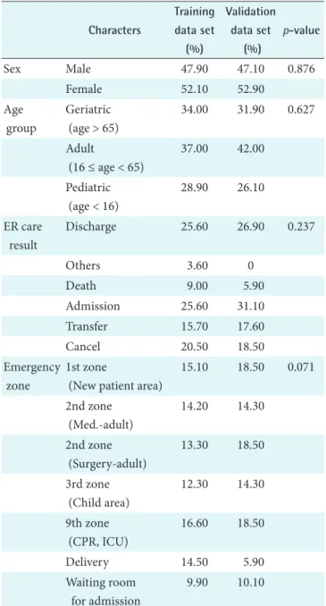
Table 2. The results of comparison between training data set and validation data set by χ² test

Characters

Training data set

(%)

Validation data set

(%)

p-value

Sex Male 47.90 47.10 0.876

Female 52.10 52.90

Age group

Geriatric (age > 65)

34.00 31.90 0.627

Adult

(16 ≤ age < 65)

37.00 42.00

Pediatric (age < 16)

28.90 26.10

ER care result

Discharge 25.60 26.90 0.237

Others 3.60 0

Death 9.00 5.90

Admission 25.60 31.10

Transfer 15.70 17.60

Cancel 20.50 18.50

Emergency zone

1st zone

(New patient area)

15.10 18.50 0.071

2nd zone (Med.-adult)

14.20 14.30

2nd zone (Surgery-adult)

13.30 18.50

3rd zone (Child area)

12.30 14.30

9th zone (CPR, ICU)

16.60 18.50

Delivery 14.50 5.90

Waiting room for admission

9.90 10.10

ER: emergency room, CPR: cardiopulmonary resuscitation, ICU: intensive care unit.

(4)

resents the relative scale of the forecasting error between the forecasted value, which is a series variable, and the observed value; the smaller the error, the more accurate the forecast is.

III. Results

Data collected from the 2007-2008 period was employed in the development of the model used to forecast the daily numbers of patients visiting the ED. The total number of patients who visitied the ED during that period was 169,375, with an annual average of 84,668 and a daily average of 232.

Chi-square tests were in order to ascertain whether any significant differences could be detected between the two datasets, and no significant differences were detected at a confidence interval of 95% (Table 2).

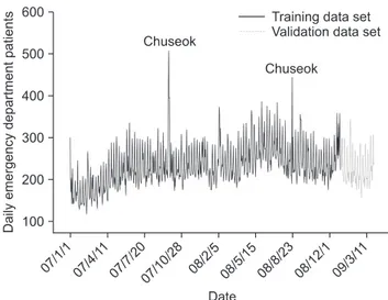
The time series diagram shows that the number of patients per day begins to increase on Saturday and peaks on Sunday, and then begins to decrease on Monday and stays low until Friday, thus describing a 7-day cycle (Figure 1).

That diagram also demonstrates that the number of visiting patients over time trends upward. The 1st seasonal difference was applied to remove the seasonal trend. As a consequence, the time series diagram suggests a stationary time series, in which the mean and deviation could not be observed clearly (Figure 2).

Three models—the MA(2) for the moving average model, SARIMA(1,0,1)(0,1,1)7 for the univariate SARIMA model

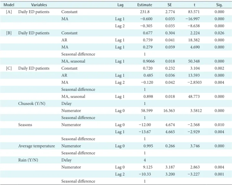
and SARIMA(1,0,2)(0,1,1)7 for the multivariate SARIMA model--were constructed using the SPSS Time Series Mod- eler. Parametric estimations using the maximal likelihood method showed that only the variables Chuseok, seasons (spring, summer, fall, and winter), average temperature, and rain could be selected as explanatory variables for the multivariate SARIMA model (Table 3).

Residual analysis for the purpose of determining the adequacy of the constructed models shows that the univariate SARIMA model and the multivariate SARIMA model, respectively, have an average of residuals that moves randomly but us centered on 0, and that the constant deviations and autocorrelation functions fall within the confidence interval, thereby indicating that the residuals are independent and fulfill the ‘white noise’ criterion.

The diagram that compares the forecasted and observed values over three months in the three forecasting models shows that the MA(2)’s forecast virtually displays the mean of the observed value, thus reflecting its inadequacy as a prediction model (Figure 3).

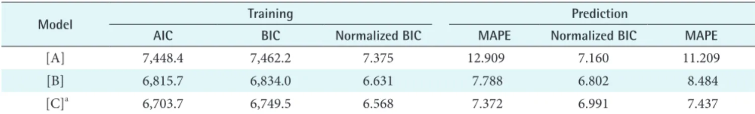
On the contrary, the SARIMA model exhibits a pattern of change similar to the observed values. Superficially, it is dif- ficult to distinguish between the univariate and multivariate SARIMA models. The AIC and BIC values, which compare the adequacy of the models, are better in the ARIMA model than in association with the moving average method, with the SARIMA(1,0,2)(0,1,1)7 model evidencing more adequate results than the univariate SARIMA model (Table 4). A MAPE comparison of the accuracy of each model’s forecasting ability demonstrates that the MA(2) models scored a 12.9%, the univariate SARIMA(1,0,1)(0,1,1)7 model scored

Figure 1. Time plots of daily emergency department (ED) patients (2007. 01-2009. 03). During the period from January 2007 to March 2009, a total of 189,511 ED patients visited and average number of daily patients was 231.

The sequencing graph showed a 7-day periodicity and seasonal trend. In particular, there was a sharp in- crease in the number of patients in Chuseok.

Figure. 2. The time series after transforms using seasonal differ- ence [1].

(5)

7.8%, and the multivariate SARIMA (1,0,2)(0,1,1)7 model scored 7.4%, thus identifying the final model as the most accurate forecasting model (Table 4): the normalized BIC values for the training and test data were also presented for comparisons.

IV. Discussion

In this study, three models are developed to forecast the number of patients visiting an ED per day: [A] Moving average model: MA(2), [B] univariate seasonal ARIMA model:

SARIMA(1,0,1)(0,1,1)7, and [C] multivariate seasonal ARIMA model: SARIMA(1,0,2)(0,1,1)7. A comparison of the goodness of fit of the three forecasting models shows that

only the final two models have residuals that fall within the confidence interval.

A comparison of the models’ forecasting accuracy shows the multivariate SARIMA model (SARIMA(1,0,2)(0,1,1)7) to be the most accurate, with a MAPE of 7.4%. The two SARIMA models have a MAPE of less than 10%, thereby suggesting a high degree of accuracy. As the SARIMA models exhibit autocorrelation and the capacity to account for seasonality, they also tend to evidence accuracy higher than the moving average. It appears that the multivariate seasonal ARIMA model can forecast the number of visiting patients more accurately than the univariate model, as it incorporates explanatory variables that affect that number (Chuseok, seasons, average temperature, and absence or presence of rain).

Table 3. Model parameters

Model Variables Lag Estimate SE t Sig.

[A] Daily ED patients Constant 231.8 2.774 83.571 0.000

MA Lag 1 -0.600 0.035 -16.997 0.000

Lag 2 -0.305 0.035 -8.638 0.000

[B] Daily ED patients Constant 0.677 0.304 2.224 0.026

AR Lag 1 0.759 0.041 18.382 0.000

MA Lag 1 0.279 0.059 4.690 0.000

Seasonal difference 1

MA, seasonal Lag 1 0.9066 0.018 50.348 0.000

[C] Daily ED patients Constant 0.720 0.232 3.104 0.002

AR Lag 1 0.485 0.036 13.593 0.000

MA Lag 2 -0.120 0.042 -2.8503 0.004

MA, seasonal Lag 1 0.898 0.018 48.773 0.000

Chuseok (Y/N) Delay 1

Numerator Lag 0 58.599 16.363 3.5812 0.000

Seasons Numerator Lag 0 -12.00 4.674 -2.568 0.010

Lag 1 -13.67 4.665 -2.929 0.004

Average temperature Numerator Lag 0 0.995 0.266 3.746 0.000

Rain (Y/N) Delay 4

Numerator Lag 0 9.125 3.187 2.863 0.004

Lag 2 -10.33 3.200 -3.227 0.001

[A]: MA(2), [B]: univariate SARIMA(1,0,1)(0,1,1)7, [C]: multivariate SARIMA (1,0,2)(0,1,1)7, ED: emergency department, SARI- MA: seasonal auto-regressive integrated moving average.

(6)

Figure 3. Observed and predicted daily emergency department patients.

Batel et al. [25] previously demonstrated that the number of visiting patients peaks on Monday and continues to decrease until Sunday, whereas Lee et al. [19]. demonstrated that the number of patients per day begins to increase on Saturday and peaks on Sunday, and then begins to decline on Monday and remains low until Friday, exhibiting a 7-day cycle and a seasonal trend. This may be attributable to differences in the medical environments. Batel et al. [25]. employed walk- in-clinics that operate for 15.5 hours over the entire week.

In this study, the number of patients visiting the ED rises on Sundays and public holidays such as Seollal and Chuseok.

This is because outpatient treatments are all closed on holidays, which means that the ED does double duty.

Lee et al. [19] identified a weak correlation among the ma- xi mal, minimal, and average temperature of the day and the

number of visiting patients, and reported no differences in the number on rainy days and non-rainy days. The same is true for snowy days and non-snowy days. Spencer et al.

[17] also argued that weather has only a minimal effect on number of patients who visited an ED. This study, however, shows that the multivariate SARIMA model that incorporates multiple weather factors generates the optimal results, thus suggesting that weather, and rain in particular, affects the numbers of visiting patients. Considering that patients in Korea consist of the following three types -1) those in an emergency situation, who require immediate treatment, 2) non-emergency patients who seek treatment on holidays or at night, and 3) non-emergency patients who seek outpatient treatment without a doctor’s reference- it can be inferred that the non-emergency patients are impacted most profoundly in this situation. In fact, Hwang et al. [14] has reports that 2,276 out of 4,273 new patients (53.3%) obtain treatment at an ED. As a consequence, considering the number of non- emergency patients who visit the ED, it is necessary to take into account weather factors when constructing demand fore casting models for emergency medical centers.

It will also be necessary to develop a variety of demand forecasting models that reflect local environments, since the studies conducted thus far have failed to take into consideration local medical systems, social and cultural backgrounds, and the relevant geographical factors.

In conclusion, as the result of our comparison of the three constructed forecast models, it was determined that the mul ti- variate SARIMA model that incorporates explanatory vari ables was the most appropriate for forecasting the daily number of patients visiting the ED; this model appears to reliably and accurately forecast the number of patients admitted to the ED per day. The results of this study demonstrated that weather information, particularly temperature and rain (or the absence there of), should be considered when attempt- ing to predict the daily volume of ED patients. The proposed

Table 4. Goodness of fits for models (AIC, BIC and normalized BIC) and MAPE values of constructed models

Model Training Prediction

AIC BIC Normalized BIC MAPE Normalized BIC MAPE

[A] 7,448.4 7,462.2 7.375 12.909 7.160 11.209

[B] 6,815.7 6,834.0 6.631 7.788 6.802 8.484

[C]^a 6,703.7 6,749.5 6.568 7.372 6.991 7.437

AIC: Akaike information criterion, BIC: Bayesian information criterion, MAPE: mean absolute percentage error, [A]: MA(2), [B]:

univariate SARIMA(1,0,1)(0,1,1)7, [C]: multivariate SARIMA (1,0,2)(0,1,1)7.

aMultivariate SARIMA Model was best in performance measurements.

(7)

prediction model can be used to forecast the daily patient volume in ED, and preparing for the previously mentioned ED crowding problems regarding the allocations of staffs and resources. More detailed prediction models related to medical demands in ED on resources and easement of overcrowding can be achieved from the proposed model via more departmentalized and processed variables that affect staff supplementation, space shortages, and the diversifica- tions of test equipments.

Conflict of Interest

No potential conflict of interest relevant to this article was reported.

Acknowledgements

This research was supported by Basic Science Research Pro- gram through the National Research Foundation of Korea (NRF) funded by the Ministry of Education, Science and Technology (20090068810).

References

1. Choung DY, Cho SH, Kim SJ. A report on the environ- ment and the present condition of local emergency medical facilities in gwangju and jeollanam-do. J Korean Soc Emerg Med 2006; 17: 116-123.

2. Tandberg D, Qualls C. Time series forecasts of emergency department patient volume, length of stay, and acuity.

Ann Emerg Med 1994; 23: 299-306.

3. Seo DW, Lim KS, Moon YS, Shon YD, Jo MW, Kim W, Lee IL. Effect of the patients new emergency fee sched- ule on the pattern of emergency. J Korean Soc Emerg Med 2004; 15: 227-232.

4. Je SM, Choi YH, Park YS, Cho YS, Kim SH. How many emergency physicians does korea need? J Korean Soc Emerg Med 2005; 16: 613-619.

5. Lee US, Park KS. The users’ component satisfaction in the emergency department. J Korean Soc Emerg Med 1994; 5: 336-465.

6. Schull MJ, Vermeulen M, Slaughter G, Morrison L, Daly P. Emergency department crowding and thrombolysis delays in acute myocardial infarction. Ann Emerg Med 2004; 44: 577-585.

7. Sun BC, Adams J, Orav EJ, Rucker DW, Brennan TA, Burstin HR. Determinants of patient satisfaction and willingness to return with emergency care. Ann Emerg Med 2000; 35: 426-434.

8. Choi HS, Lee KW. Analysis of overcrowding in a local emergency department using nAtional emergency department overcrowding scale (NEDOCS). J Korean Soc Emerg Med 2006; 17: 377-384.

9. Derlet RW, Richards JR. Overcrowding in the nation’s emergency departments: complex causes and disturbing effects. Ann Emerg Med 2000; 35: 63-68.

10. Arnold JL, Song HS, Chung JM. The recent development of emergency medicine in South Korea. Ann Emerg Med 1998; 32: 730-735.

11. Jung KY, Lim KS, Min YI, Lee SB, Kim SK. The present status of emergency care in emergency centers. J Korean Soc Emerg Med 1997; 8: 441-459.

12. Schweiger L, Younger J, Ionides E, Desmond J. Au- toregression models can reliably forecast emergency depart ment occupancy levels 12 hours in advance. Acad Emerg Med 2007; 14: S82.

13. Jones SS, Evans RS, Allen TL, Thomas A, Haug PJ, Welch SJ, Snow GL. A multivariate time series approach to mo deling and forecasting demand in the emergency department. J Biomed Inform 2009; 42: 123-139.

14. Hwang SW, Lee HJ. Development of a revisit prediction model for the outpatient in a hospital. J Korean Soc Med Inform 2008; 14: 137-145.

15. Schweigler LM, Desmond JS, McCarthy ML, Bukowski KJ, Ionides EL, Younger JG. Forecasting models of emergency department crowding. Acad Emerg Med 2009; 16:

301-308.

16. Asplin BR, Flottemesch TJ, Gordon BR. Developing models for patient flow and daily surge capacity research. Acad Emerg Med 2006; 13: 1109-1113.

17. Jones SS, Thomas A, Evans RS, Welch SJ, Haug PJ, Snow GL. Forecasting daily patient volumes in the emergency department. Acad Emerg Med 2008; 15: 159-170.

18. Sun Y, Heng BH, Seow YT, Seow E. Forecasting daily at- tendances at an emergency department to aid resource planning. BMC Emerg Med 2009; 9: 1.

19. Lee JY, Min JH, Park JS, Chung SP, Park JS, Jung SK, Yang YM. The association of meterological and day-of- the week factors with patient visits to emergency centers. J Korean Soc Emerg Med 2005; 16: 287-291.

20. Korea Meteorological Administration; c2009 [cited at 2009 April 20]. Available from: http://www.kma.go.kr/.

21. Do JD. A study the change point of stock price. J Inst Nat Sci 2007; 25: 27-34.

22. Yi KH, Chung HK, Park JS. The prediction model of the number of industrial injured persons using data mining.

Korean J Occup Environ Med 2000; 12: 515-523.

23. Akaike H. A new look at the statistical model identifica-

(8)

tion. IEEE Trans Automatic Control 1974; 19: 716-723.

24. Schwarz G. Estimating the dimension of a model. Ann Statist 1978; 6: 461-464.

25. Batal H, Tench J, McMillan S, Adams J, Mehler PS. Pre- dicting patient visits to an urgent care clinic using calendar variables. Acad Emerg Med 2001; 8: 48-53.