USING REMOTE SENSING AND PURSE SEINE CATCH DATA TO DETECT OCEAN HOT SPOTS FOR YELLOWFIN TUNAS IN THE
TROPICAL PACIFIC OCEAN
Kuo-Wei Yen*, Hsueh-Jung Lu and Ming-An Lee
Department of Environmental Biology and Fisheries Science, National Taiwan Ocean University 2 Pei-Ning Rd, 20224, Keelung, Taiwan. [email protected]
ABSTRACT In this study, we analyzed catch data of Taiwan tuna purse seines fishery and remotely sensed oceanographic data, including sea surface temperature (SST), chlorophyll-a (SSC), height anomaly (SSH) and salinity (SSS), in order to locate hot spots for yellowfin tunas (YFT). Hot spots, defined as the areas with relatively high occurrence of purse seining activities and YFT catch, were determined by empirical model. To establish such model, daily catch data during 2003-2007 were aggregated monthly into 1 by 1 degree and then conduct data match process to obtain monthly average values for the 4 factors (SST, SSC, SSH and SSS) where harvest took place. As the frequency distribution of the each factor on which YFT caught performed normal distributions pattern, we then transformed the values of the 4 factors into Habitat Suitability Index (HI), i.e. from low to high (1-4). With these empirical HI formed during 2003~2007, weighted HI by month with single as well as multiple factors were then computed to predict monthly hot spots for YFT. We used GIS overlay technique to test the predictability and the results were encouraging.
The correct prediction rate for YFT hot spot by single factors are about 53%-68%, among them SST is the most powerful predictor followed SST, SSC, SSS and SSH. The predictability can be raised up to 77% if all factors were applied. However, the predictability during the period varied month by month and year after year. This study also discussed the possible reasons resulting in the fluctuation of the predictability.
KEY WORDS: Sea surface temperature, chlorophyll-a, sea surface height anomaly, sea surface salinity, purse seine, yellowfin tuna,Habitat suitability index
1. INTRODUCTION
Yellowfin tuna (YFT) Thunnus albacores (Bonnaterre, 1788) distributes extensively in open waters of tropical and subtropical oceans. About 85%
of time during a day. YFT like to stay in shallow layer less than 75 meters (Laurent et al., 2006), where environmental factors were relatively sensitive and resulted in complicated migration behaviour to react high vertical variation of current, temperature, salinity and bait (Keith et al., 1997; Juan Antonio et al., 2004).
The information of remote sensing has been widely applied to fishery research, including sea surface temperature (SST), sea surface chlorophyll-a (SSC), sea surface height anomaly (SSHA) and sea surface salinity (SSS) (Romena, 2001; Zhang et al., 2001;
James et al., 2005; Zainuddin et al., 2008). These factors obtained by remote sensing have been successfully applied to develop habitat suitability index (HI) for many kinds of marine fishes (Palm et al., 2009; Chen et al., 2009; Daugherty et al., 2008;
Haxton et al., 2008). However, until now there were no related studies carried on the HI for YFT.
Almost 70 percent of total tuna catch in the western and central Pacific (WCPO) is from purse seine fishery and YFT makes up 15 percent of total tuna in the WCPO.
The main objective of this study is to understand the preference ranges of the factors obtained from remote sensing in the WCPO, so as to develop algorithm of HI to detect hot spots for YFT in such region. We also discuss about the shift of HI in space and time during different climatic periods i.e. El Niño, La Niña and Normal.
2. MATERIAL AND METHOD
2.1 Data
Four categories of data were collected in this study including YFT catch and effort data, SST, SSC, SSHA, SSS and Southern Oscillation index (SOI):
1. Catch and effort data of Taiwanese purse seiners during 2003~2007 were provided by the Overseas Fishery Development Council of the Republic of China, including fishing locations, effort, catch, time and school type.
2. Monthly SST and SSC were taken from NASA MODIS Satellite Imagery. The data is in HDF format covering areas from 10°S to10°N and 135°E to150°W with pixel resolution of 4km.
3. Daily data sets of SSHA and SSS were taken from Oceanography Division of the U.S. of Naval Research Laboratory; the data is in GIF format covering areas from 10°S to10°N, 135°E to150°W at a pixel resolution of 1/8°.
4. SOI was taken from NOAA Climate Analysis Center, which is defined as gradient average of atmospheric pressure (mb) between Tahiti and Darwin.
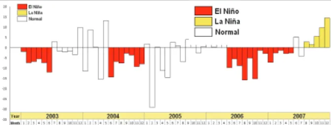
In this study, if negative SOI values lasted for 6 months, we defined the periods as El Niño. If positive SOI values lasted for 6 months, we defined them as La Niña periods. The other were then defined as normal periods (Figure 1)
Figure 1. El Niño and La Niña period during 2003-2007 were determined by SOI, the monthly atmospheric pressure difference at sea level between Tahiti and Darwin.
2.2 The spatial distribution of YFT hot spots
In order to understand the hot spots distribution of YFT, we collects catch and effort data as we
mentioned above, then add up all the high YFT catch data (i.e. CPUE > 1 ton) in each month of each latitude-longitude grid.
The monthly hot spot for the fish in 1°×1° grid was calculated as follows:
Where i =longitude, j =latitude, m=month, y =year.
2.3 Extraction of HV on fishing locations
Interactive data language (IDL) and Visual Basic (VB) were used to develop programs for extraction process.
Four habitat variables (SST, SSC, SSHA and SSS) at the locations where and when a fishing operation took place were extracted one by one from HDF and GIF images, respectively.
2.4 Habitat suitability index
We computed HI for YFT from habitat variables (HV) extracted from the location with high YFT catch. The value for each HV were transformed into nominal variables by quartile (1-4), was calculated as follows:
Where X= environment parameter.
= measurement for satellite-derived oceanographic variables from the high YFT catch fishing trip i.
S = standard deviation of all . = average of all .
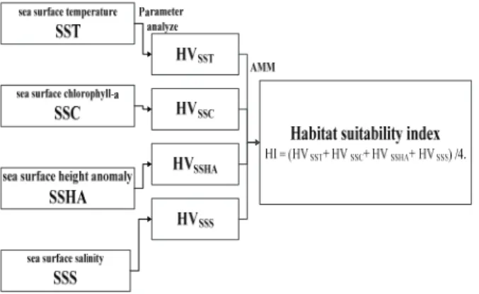
We adopted Arithmetic Mean Model (AMM) (Hess and Bay, 2000; Xinjun et al., 2009) to compute HI by the 4 HVs (Figure 2).
Figure 2. Diagram showing the procedure of habitat suitability index determination.
3. RESULT
3.1 Optimum range of SST for YFT
As shown in Figure 3, we found that YFT was widely distributed in waters with SST ranging from 27.28-32.43 , ℃ and centralization tendency distributed at 30.8℃. There are no significant differences on SST distribution among 3 school types (Figure 3), which means different school types has similar favour on selecting SST. Besides, we realized that climate types affected SST greatly, however, there seems no centralization tendency changes in the distribution of SST (Figure 4). Hence, the movement of purse seine fleet is rapid enough to catch up the movement of YFT habitat.
Figure 3. Frequency distribution of SST for three tyoes of schooling YFT canght during 2003-2007.
Figure 4. Frequency distribution of SST where high YFT catch under three climate types during 2003-2007.
3.2 Optimum range of SSC for YFT
YFT prefer to distribute in waters with SSC ranging from 0.02- 0.30mg/m3 with average value about 0.07 mg/m3(Figure 5). Like the pattern revealed by SST preference, we found that there is no significant differences of SSC between among three YFT school type. An interesting phenomenon is that the distribution area with SSC value lower than 0.06 mg/m3 increase evidently while El Niño phenomenon prevalent.
Conversely, the distribution areas with SSC value over 0.06 mg/m3 increase obviously in La Niña (Figure 6).
Figure 5. Frequency distribution of SSC for three types of schooling YFT canght during 2003-2007.
Figure 6. Frequency distribution of SSC where high YFT catch under three climate types during 2003-2007.
3.3 Optimum range of SSHA for YFT
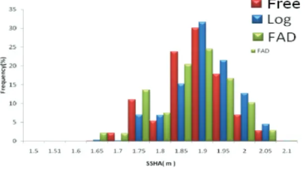
There are no difference of SSHA preference among schooling types (Figure 7). However, the abnormal climate will affect YFT's preference of inhabit. The SSHA rang from 1.51-2.1m, with peaks at 1.9 and 1.95 during El Niño periods and SSHA rang from 1.75-1.95m, with a peak value at 1.85m during La Niña period. The SSHA value in normal climate period seems to be similar to La Niña case. (Figure 8)
Figure 7. Frequency distribution of SSHA for three types of schooling YFT canght during 2003-2007.
Figure 8. Frequency distribution of SSHA where high YFT catch under three climate types during 2003-2007.
3.4 Optimum range of SSS for the YFT
The preference ranges of SSS about 34.2-3.54 psu, with peak at 34.6 psu. Free schools prefer to inhabit at SSS value of 34.6 psu. However, FAD school has wider SSS range then the other two (Figure 9). Furthermore, we found that there are significant differences of SSS among three climate school types (Figure 10).
Figure 9. Frequency distribution of SSS for three types of schooling YFT canght during 2003-2007.
Figure 10. Frequency distribution of SSS where high YFT catch under three climate types during 2003-2007.
3.5 HI and YFT high catch regional
As the frequency distribution of each factor where YFT caught performed normal distributions pattern, we then transformed the values of the 4 factors into HV, i.e.
from low to high (1-4). Since there are no significant differences on three YFT school types when selecting
inhabit, we only consider the climate types as the main influential parameter when conducting calculation of HI.
Empirical HI models for three climate types were developed. With these empirical HI formed during 2003~2007, weighted HI by month with single as well as multiple factors were then computed to predict monthly hot spots for YFT. We used GIS overlay technique to test the predictability and the results were encouraging. The correct prediction rate for YFT hot spot by single factors are about 53%-68%, among them SST is the most powerful predictor followed SST, SSC, SSS and SSH. The predictability can be raised up to 77% if all factors were applied.
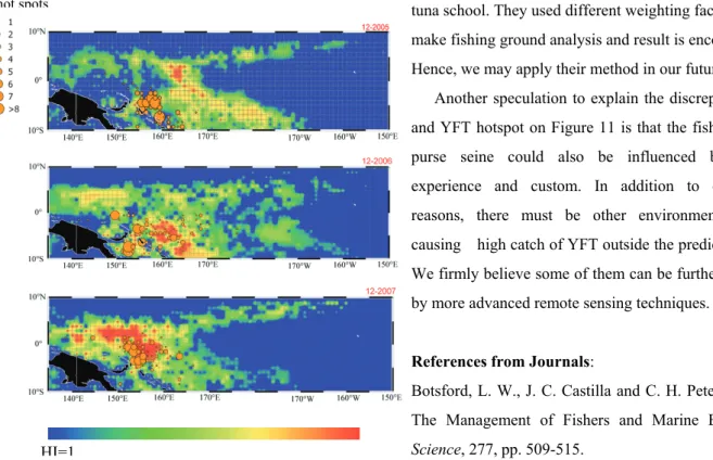
Figure11 showed examples of HI distribution by AMM model and real spatial distribution of YFT from purse-seine fishery in three Decembers of different climate scenario (2005= Normal; 2006= El Niño;
2007=La Niña). The predicted hot spots by the AMM with 4 HVs indicated that high consistency of predicted HI and YFT hot spot from purse seines.
Figure 11. The spatial distribution of YFT hot spots from purse seines in three climate types: Normal (12-2005), El Niño (12-2006), La Niña (12-2007) overlaid on predicted HI by the AMM using the 4 HVs (SST, SSC, SSHA and SSS).
4. DISCUSSION AND CONCLUSION
The four factors used in this study have been proven to be valid not only for YFT but also in detecting potential forage habitats for pelagic species (Polovina et al., 2001, 2004). In this study we used short time series data sets (2003–2007) and only selected four
environmental factors obtained from remote sensing database to define the environmental features of YFT hot spots. However, AMM model applied in this study is subjective as all factors are equally weighted which may distort the fact. We should make multi-vitiate analysis on all factors before determining weighted HI for YFT. In year 2008, Zainuddin et al. published an intensive study about how powerful the environment factors affect the tuna school. They used different weighting factors to make fishing ground analysis and result is encouraging.
Hence, we may apply their method in our future study.
Another speculation to explain the discrepancy of HI and YFT hotspot on Figure 11 is that the fishing area of purse seine could also be influenced by fishers’
experience and custom. In addition to commercial reasons, there must be other environmental factors causing high catch of YFT outside the predicted region.
We firmly believe some of them can be further explained by more advanced remote sensing techniques.
References from Journals:
Botsford, L. W., J. C. Castilla and C. H. Peterson, 1997.
The Management of Fishers and Marine Ecosystems.
Science, 277, pp. 509-515.
HI=1 HI=4
hot spots
Brander, K. M., 2007. Gobal fish production and climate change. Proceedings of the National Academy of Sciences, 104, pp. 19709-19714.
Cui, K. and X. J. Chen, 2005. Study on inter-annual change of the yields of Pnunmatophorus japonicus and Decapterus maruadsi for purse seine fishing grounds in the East China Sea and the Yellow Sea. Donghai Marine Science, 23(2), pp. 41–49.
Daugherty D.J., Sutton T.M., Elliott R.F., 2008.
Potential for reintroduction of lake sturgeon in five northern Lake Michigan tributaries: a habitat suitability perspective. Aquatic Conservation:
Marine and Freshwater Ecosystems, 18 (5), pp.
692-702.
Haxton T.J., Findlay C.S., Threader R.W., 2008.
Predictive Value of a Lake Sturgeon Habitat Suitability Model. North American Journal of Fisheries. Management, 28 (5), pp. 1373-1383.
Hess, G. R. and J. M. Bay, 2000. A regional assessment of windbreak habitat suitability.
Environmental Monitor Assessment, 6(12), pp.
239–256.
Hiyama, Y., M. Yoda and S. Ohshimo, 2002. Stock size fluctuations in Chub mackerel (Scomber japonicus) in the East China Sea and the Japan.
Fisheries Oceanography., 11, pp.347–353.
De Anda-Montanez J.A., Amador-Buenrostro A., Martinez-Aguilar S., Muhlia-Almazan A., 2004.
Spatial analysis of yellowfin tuna (Thunnus albacares) catch rate and its relation to El Niño and La Niña events in the eastern tropical Pacific. Deep-Sea Research, II (51), pp. 575–586
Korsmeyer, K.E., Lai, N.C., Shadwick, R.E., and Graham, J.B.,1997. Heart rate and stroke volumecontributions to cardiac output in swimming yellowfin tuna: response to exercise and temperature.
Journal of Experimental Biology, 200(14), pp.
1975-1986
Dagorn L, Holland KN, Hallier JP, Taquet M., Moreno G., Sancho G., Itano D.G., Aumeeruddy R., Girard C., Million J., Fonteneau A., 2006. Deep diving behavior observed in yellowfin tuna (Thunnus albacares). Aquatic Living Resources. 19, pp. 85–88
Zainuddin M., Saitoh K. , Saitoh S.-I., 2008. Albacore (Thunnus alalunga) fishing ground in relation to oceanographic conditions in the western North Pacific Ocean using remotely sensed satellite data. Fisheries Oceanography, 17(2), pp. 61–73.
Palm D., Brannas E., Nilsson K., 2009. Predicting site-specific overwintering of juvenile brown trout (Salmo trutta) using a habitat suitability index.
Canadian Journal of Fisheries and Aquatic Sciences, 66 (4), pp. 540-546.
Polovina, J.J., Balazs, G.H., Howell, E.A., Parker, D.M., Seki, M.P. and Dutton, P.H., 2004. Forage and migration habitat of loggerhead (Caretta caretta) and olive ridley (Levidochelys olivacea) sea turtles in the central North Pacific Ocean. Fisheries Oceanography, 13, pp. 36–51.
Polovina, J.J., Howel, E., Kobayashi, D.R. and Seki, M.P., 2001. The transition zone chlorophyll front, a dynamic global feature defining migration and forage habitat for marine resources. Progress in Oceanography, 49, pp.
469–483.
Brill R.W., Block B.A., Boggs C.H., Bigelow K.A., Freund E.V., Marcinek D.J., 1999. Horizontal movements and depth distribution of large adult yellowfin tuna (Thunnus albacares) near the Hawaiian Islands, recorded using ultrasonic telemetry: implications for the physiological ecology of pelagic fishes. Marine Biology. 133, pp. 395-408
Romena, N.A., 2001. Factors affecting distribution of adult yellowfin tuna (Thunnus albacares) and its reproductive ecology in the Indian Ocean based on Japanese tuna longline fisheries and survey information.
International Offshore Technology Committee Proc.4, pp. 336–389.
Sun, C. H., F. S. Chiang and E. T. Soac, 2006. The effects of El Niño on the mackerel purse-seine fishery harvests in Taiwan: An analysis integrating the barometric readings and sea surface temperature.
Ecological Economics, 56, pp. 268–279.
Tilstone G. , Smyth T. , Poulton A., Hutson R., 2009.
Measured and remotely sensed estimates of primary production in the Atlantic Ocean from 1998 to 2005.
Deep Sea Research Part II: Topical Studies in Oceanography, 56 (15), pp. 918-930.
Wang ZM., Liu ZM., Song KS., Zhang B., Zhang SM., Liu D.W., Ren C.Y., Yang F., 2009. Land use changes in Northeast China driven by human activities and climatic variation. Chinese Geographical Science, 19(3), pp. 225-230.
Chen X.J., Li G., Feng B., Tian SQ., 2009. Habitat Suitability Index of Chub Mackerel (Scomber japonicus) from July to September in the East China Sea. Journal of Oceanography, 65, pp. 93-102.
Yatsu, A., T. Watanabe, M. Ishida, H. Sugisaki and L.
D. Jacobson, 2005. Environmental effects on recruitment and productivity of Japanese sardine Sardinops melanostictus and Chub mackerel Scomber japonicus with recommendations for management.
Fisheries Oceanography, 14, pp. 263–278.
Yatsuia, A., T. Mitana, C. Watnabe, H. Nishida, A.
Kawabata and H. Matuuda, 2002. Current stock status and management of Chub mackerel, Scomber japonicus, along the Pacific coast of Japan—an example of allowable biological catch determination.
Fisheries Science, 68 (Suppl. I) , pp.93–96.
References from Books:
Smith, J., 1989. Oceanology. Universities Press, India, pp.44.
James L Sumich, Gordon Dudley, 2005. Laboratory and field investigations in marine life. Jones & Bartlett, Sudbury, Mass., pp.39.
References from Other Literature:
Western and Central Pacific Fisheries Commission, 2008.
Tuna Fishery Yearbook 2007.
Western and Central Pacific Fisheries Commission, 2006, Stock assessment of yellowfin tuna in the western and central Pacific Including Analysis of Management Options.