Evaluating Interval Estimates for Comparing Two Proportions with Rare Events

(1)

Evaluating Interval Estimates for Comparing Two Proportions with Rare Events

Jin-Kyung Park

¹

· Yongdai Kim

²

· Hakbae Lee

³

1

International Vaccine Institute;

²

Department of Statistics, Seoul National University

3

Department of Applied Statistics, Yonsei University

(Received April 2, 2012; Revised April 22, 2012; Accepted April 30, 2012)

Abstract

Epidemiologic studies frequently try to estimate the impact of a specific risk factor. The risk difference and the risk ratio are generally useful measurements for this purpose. When using such measurements for rare events, the standard approaches based on the normal approximation may fail, in particular when no events are observed. In this paper, we discuss and evaluate several existing methods to construct confidence intervals around risk differences and risk ratios using Monte-Carlo simulations when the disease of interest is rare. The results in this paper provide guidance how to construct interval estimates of the risk differences and the risk ratios when no events are detected.

Keywords: Bayesian probability interval, conﬁdence interval, rare events, risk ratio, risk diﬀerence.

1. Introduction

In epidemiologic research estimates of disease frequency are the basis for the comparison of populations and the identification of disease determinants. The comparison of two frequencies can be combined into a single summary parameter that estimates the association between an exposure and the risk of developing a disease. This can be accomplished by calculating the risk difference and the risk ratio. The risk difference(RD) is defined as the difference between the risk in the exposed and non-exposed groups and provides information about the absolute effect of the exposure or the excess risk of disease in those exposed over those non-exposed. The RD describes the absolute change in risk attributable to the exposure and is useful in answering the question how much of the disease can be prevented if the exposure in question is eliminated. In epidemiology a more frequent measure of the difference between two proportions is their ratio referred to as the risk ratio, rate ratio, or relative risk, depending on the type of study. A risk ratio(RR) or relative risk is the ratio of the incidence of disease in the exposed group divided by the corresponding incidence of disease in the non-exposed group.

Both RD and RR can be used to determine the existence and the strength of an association between exposure and outcome in cohort studies but are not appropriate for the analysis of case-control

3Corresponding author: Associate professor, Department of Applied Statistics, Yonsei University, 50 Yonsei- ro, Seodaemun-gu, Seoul 120-749, Korea. E-mail: [email protected]

(2)

studies. Instead, the odds ratio(OR) is used in case-control studies, another measurement of the association between exposure and outcome. The OR is often referred to as approximate relative risk because the OR can be used as an estimate of RR when the incidence of disease is very low.

Suppose x

1

and x

2

are disease frequencies of two independent populations with sizes n

1

and n

2

respectively. The RD and the RR are deﬁned by p

1

− p

2

and p

1

/p

2

respectively where p

1

and p

2

are the probabilities of disease in two populations. The standard methods of constructing conﬁdence interval(CI) of RD and RR are based on normal approximation, these are used widely in most of statistical software packages by non-statisticians. Along with the computational simplicity, the CI of RD has an apparent advantage of producing interval centered on the point estimate, thus resembling one for the mean of a continuous normal variate. In addition, the CI of RR generally has the asymptotic normality of the natural logarithm of an observed ratio.

However, when x

1

= x

2

= 0, we have a problem with using the interval estimates of RD and RR.

The CI of RD is zero length, and the CI of RR is not deﬁned. The situation in which no cases occur in a binomial experiment arises quite frequently when p

1

and p

2

are small. Examples are an epidemiologic study where disease of interest is a rare event and a diagnostic test in which it is common to deal with a small false negative rate (the probability of a disease individual testing negative). Newcombe (1998a, 1998b) has studied interval estimation of single proportion and the difference of two independent proportions. Newcombe (1998b) examined risk differences(RDs) in symmetry and aberrations as well as degree of coverage based on various sample parameter space points. Two types of aberrations are classified based on the location of the interval and the expected interval width as tethering and overt overshooting. Tethering occurs if either the calculated upper and lower limits coincide with the point estimate. Overt overshooting occurs if either calculated limit is outside the boundaries. These aberration problems can occur in the analysis of rare events.

Various approaches to interval estimation of the RD have been proposed by Santner and Snell (1980), Beal (1987), Mee (1984), Miettinen and Nurminen (1985) and Newcombe (1998b). Approaches to RR estimation have been evaluated by Noether (1957), Walter (1975), Katz et al. (1978), Aitchison and Bacon-Shone (1981), Koopman (1984), Mee (1984), Miettinen and Nurminen (1985), Gart and Nam (1988), and Ewell (1996).

All of these studies focused on improving the performances of interval estimates in studies with a small sample size. Chan (1998) proposed exact tests of equivalent and eﬃcacy that are desirable for studies with small sample sizes. To our knowledge, our simulation experiment is the ﬁrst comparative study for interval estimates of the RD and the RR with small probabilities of the disease case.

This paper discusses interval estimates, the CI of RD and RR, when there is a small probability of a disease under investigation to occur. In contrast to the p-value the use of the CI to interpret a result has the advantage that the CI is measured with the same scale of data while the p-value is a probabilistic measurement. The CI conveys information about magnitude and precision of eﬀect.

A point estimate is of limited value without some indication of its precision. This is provided by the CI (Newcombe, 1998a).

Our paper is divided in 4 sections. In the following Section 2, we describe interval estimates for

RD and RR. In Section 3 examples are shown to highlight problems. Simulation results using

Monte-Carlo methods are provided in Section 4. The ﬁndings are discussed at the end of the paper.

(3)

2. Various Interval Estimates 2.1. Risk diﬀerence

Newcombe (1998b) evaluated several existing methods to estimate the CI for the difference between two proportions. He concluded that the profile likelihood based method produces the best coverage probabilities, though it may be difficult to calculate for a large denominator. The Wilson score method is known to have good coverage probabilities for small and medium size data. In this subsection, we will describe four RD interval estimates (that include profile likelihood based and Wilson score method) that in most circumstances perform well. A simple asymptotic method used in most software packages (the Wilson score method, the exact method, and the Bayesian probability method) are discussed here. When the number of observations is small, the exact method has the same logic framework as the profile likelihood based method familiar to StatXact users. The exact method of StatXact is used in this paper as an alternative of profile likelihood based method. The Bayesian probability method is included because it yields the interval estimates of a proportion in a one sample problem close to the exact confidence interval when no cases are observed (Louis, 1981).

1. Normal approximation(NA)

The interval estimate of RD based on the normal approximation is given as (ˆ p

1

− ˆp

2

) ± z

^α₂

√ p ˆ

1

(1 − ˆp

1

) n

1

+ p ˆ

2

(1 − ˆp

2

) n

2

, (2.1)

where ˆ p

1

= x

1

/n

1

and ˆ p

2

= x

2

/n

2

. This method gives good results for large prospective studies, while these limits yield an interval of (0, 0), a tethering when x

1

= x

2

= 0.

2. Wilson score method(WS)

The 100(1 − α)% conﬁdence interval (L, U) of the Wilson score method is given as

L = ˆ p

1

− ˆp

2

− δ, U = ˆp

1

− ˆp

2

+ ϵ (2.2) where

δ =

√( x

1

n

1

− l

1

)

2

+ (

u

2

− x

2

n

2

)

2

= z

^α

2

√ l

1

(1 − l

1

) n

1

+ u

2

(1 − u

2

) n

2

,

ϵ =

√(

u

1

− x

1

n

1

)

2

+ ( x

2

n

2

− l

2

)

2

= z

^α

2

√ u

1

(1 − u

1

) n

1

+ l

2

(1 − l

2

) n

2

,

l

1

and u

1

are the roots of |p

1

− x

1

/n

1

| = z

α/2

√ p

1

(1 − p

1

)/n

1

, and l

2

and u

2

are the roots of

|p

2

− x

2

/n

2

| = z

α/2

√ p

2

(1 − p

2

)/n

2

(Wilson, 1927). When x

1

= x

2

= 0, they are 0 = l

1

< u

1

< 1 and 0 = l

2

< u

2

< 1 and δ and ϵ become u

2

and u

1

respectively. Therefore, (L, U ) of the Wilson score method have no aberrations.

3. Exact method(EX)

Let θ = p

1

− p

2

and ψ = p

2

. Consider a test of H

0

(x) : p

1

− p

2

= x versus H

1

: p

1

− p

2

̸= x. We reject H

0

(x) when |ˆp

1

− ˆp

2

− x| is larger than the critical value C

x

. If we know the true value of ψ, then the critical value C

x

is calculated for a given level α by

Pr{|ˆp

1

− ˆp

2

− x| > C

x

|θ = x, ψ} = α

2 . (2.3)

(4)

Now, we can construct the exact 100(1 − α)% conﬁdence interval (L, U) by L = inf{x : H

0

(x) is not rejected},

and

U = sup {x : H

0

(x) is not rejected }.

See Bickel and Doksum (1977, p.155). However, we don’t know ψ. One simple remedy for this problem is to eliminate nuisance parameter ψ by taking supremum over its range suggested by Santner and Snell(1980). Berger and Boos(1994) suggested a modiﬁed method of searching supremum and eliminating in a restricted range. As a ﬁrst step, an exact 100(1 − γ)% intervals for p

1

and p

2

are computed. Denote those intervals as A

1

= [l

1

, u

1

] and A

2

= [l

2

, u

2

] respectively. Assume that the event ε : (p

1

, p

2

) ∈ A

1

× A

2

is true. Then 100(1 − α)% exact conﬁdence interval (L, U) in restricted range (l

2

− u

1

, u

2

− l

1

) is given that satisﬁes the conditions

sup

ψ∈ε^∗

Pr (ˆ p

1

− ˆp

2

≤ x|L = x, ψ) = α 2 − γ, sup

ψ∈ε^∗

Pr (ˆ p

1

− ˆp

2

≥ x|U = x, ψ) = α 2 − γ, where ε

^∗

= {p

2

: max(l

2

, l

1

− x) ≤ p

2

≤ min(u

2

, u

1

− x)}.

The intervals (l

i

, u

i

), (i = 1, 2) are calculated within (0, 1) from the two independent binomial distributions and the interval (L, U ), as mentioned, is always in restricted range (l

2

− u

1

, u

2

− l

1

), which is narrower than boundary ( −1, 1). This modiﬁed method can provide stability, narrower CI, and faster execution by cutting of regions near the extremes of the parameter space.

4. Bayesian probability method(BP)

The Bayesian probability interval of RD is constructed as follows. Let π(p

1

, p

2

) be the prior distribution of (p

1

, p

2

). Then the posterior distribution is given by

π(p

1

, p

2

|x

1

, x

2

) ∝ p

^x1¹

(1 − p

1

)

ⁿ¹^−x¹

p

^x₂²

(1 − p

2

)

ⁿ²^−x²

π(p

1

, p

2

).

Let θ = p

1

− p

2

and ψ = p

1

+ p

2

, and let π(θ, ψ |x

1

, x

2

) be the corresponding posterior distribution of θ and ψ, which can be obtained by using the variable transformation technique. Now, the equal tail 100(1 − α)% probability interval has the form of (L, U) which satisﬁes

∫

₁

U

∫

₂

0

π(θ, ψ |X

1

, X

2

)dψdθ = α 2 and

∫

L

−1

∫

2 0

π(θ, ψ|X

1

, X

2

)dψdθ = α 2 .

See Gelman et al. (1995). In practice, we can obtain L and U by using a simple Monte-Carlo method as follows. First, we generate p

1

and p

2

from their posterior distributions and calculate θ = p

1

− p

2

. We repeat this several times to get many θs generated from the posterior distributions.

Finally, L and U are obtained from the histogram of θs.

(5)

2.2. Risk Ratio

Gart and Nam(1988) grouped several RR interval estimates into three categories based on their mode of derivation, which are the normal approximate methods, the Fieller-like method, and the likelihood based method. In this subsection, we brieﬂy describe these three methods along with the Bayesian probability method.

1. Normal approximation(NA)

There are two approaches to construct the CI of RR; the delta method and the exponential transformation. The delta method is to compute the CI of RR using delta rule to derive an estimate of standard error(SE) while the exponential transformation method is to transform RR exponentially to approximate normal, then transformed end-points of the CI in the natural parameter space.

Asymptotically, these two are equivalent; however, they will diﬀer for real data.

The 100(1 − α)% CI by using delta method is ˆ

p

1

ˆ p

2

( 1 ± z

^α₂

√ 1 − ˆp

1

n

1

p ˆ

1

+ 1 − ˆp

2

n

2

p ˆ

2

)

, (2.4)

where ˆ p

1

= x

1

/n

1

and ˆ p

2

= x

2

/n

2

.

In practice, the CI obtained by transforming the end-points has some intuitively desirable properties, for example, they do not produce negative RR. In general, we also expect the estimates to be more normally distributed. The 100(1 − α)% approximate CI of RR used in this paper is one using the exponential transformation method and is given as

exp [

(log(ˆ p

1

) − log(ˆp

2

)) ± z

^α₂

√ 1 − ˆp

1

n

1

p ˆ

1

+ 1 − ˆp

2

n

2

p ˆ

2

]

, (2.5)

where ˆ p

1

= x

1

/n

1

and ˆ p

2

= x

2

/n

2

. The limits are not deﬁned when either or both of x

1

and x

2

are zero.

2. Fieller-like method(FL)

Denote ϕ = p

1

/p

2

. The Fieller-like interval uses the statistic T = ˆ ϕ − ϕ where ˆϕ = ˆp

1

/ˆ p

2

. It can be shown that T is asymptotically normal with variance

var(T ) = ϕ

²

q

2

n

2

p

2

+ ϕ

²

q

1

n

1

p

1

.

p

1

in this variance formula is substituted by ϕp

2

and p

2

is estimated by ˆ p

2

. Finally, the 100(1 − α)%

conﬁdence interval using this estimated variance V (T ) is given as the solution of following quadratic equation;

( ϕ ˆ − ϕ )

2

= z

²^α

2

V (T ). (2.6)

This Fieller-like interval estimate is proposed by Noether (1957). A diﬀerent type of Fieller-like interval estimates for RR based on the statistic T

^′

= ˆ p

1

− ϕˆp

2

has been proposed by Katz et al.

(1978). If both x

1

and x

2

are greater than zero, the equation always yields real roots. However,

when x

2

= 0 the variance and the point estimate ˆ ϕ are not deﬁned. When x

1

= 0 and x

2

̸= 0, one

limit becomes zero, which is a tethering and the other limit may be less than zero. When ˆ p

2

is very

(6)

small, these roots may be complex or may be exclusive such like disjoint conﬁdent interval, that is, (0, a) and (b, ∞) where b > a.

3. Likelihood based method(LB)

Miettinen and Nurminen (1985) have proposed a method that uses the maximum likelihood esti- mator(MLE) of the nuisance parameter p

2

, for a given value of ϕ = p

1

/p

2

. Let ˜ p

2

be the MLE of p

2

given ϕ and let ˜ p

1

= ϕ˜ p

2

. The MLE of p

2

, ˜ p

2

is the appropriate solution to the quadratic equation a˜ p

²2

+ b˜ p

2

+ c = 0,

where a = (n

1

+ n

2

)ϕ, b = −[(x

2

+ n

1

)ϕ + x

1

+ n

2

], and c = x

1

+ x

2

. They started with the statistic T = ˆ p

1

− ϕˆp

2

and estimated its variance by ˜ p

1

q ˜

1

/n

1

+ ϕ

²

p ˜

2

q ˜

2

/n

2

. Then, they obtained the limits of 100(1 − α)% conﬁdence interval as the roots to the equation

(ˆ p

1

− ϕˆp

2

)

²

(˜ p

1

q ˜

1

)/n

1

+ (ϕ

²

p ˜

2

q ˜

2

)/n

2

( n

1

+ n

2

− 1 n

1

+ n

2

)

= z

²^α

2

. (2.7)

Koopman (1984) derived the same confidence interval from different derivation. Gart and Nam (1988) showed Miettinen and Nurminen method and Koopman’s method are identical. The only difference is that Miettinen and Nurminen use a variance correction, so the resulting limits are slightly wider than those given by Koopman’s formulation. When x

1

and x

2

are zero, the variance is not deﬁned because the MLE of the nuisance parameter p

2

becomes zero. If either x

1

or x

2

is zero, only one limit is found because the left term of (2.7) does not be quadratic for ϕ > 0.

4. Bayesian probability method(BP)

The Bayesian probability approach for RR is very similar to one for RD. First, we calculate the posterior distribution of (p

1

, p

2

) and obtain the posterior distribution of p

1

/p

2

by use of the variable transformation technique. Finally, we get limits of the equal tail 100(1 −α)% probability interval as the upper and lower 100(α/2) percentiles of the posterior distribution of p

1

/p

2

. In addition, these percentiles can be calculated easily using the simple Monte-Carlo method as is done for RD.

3. Examples

In this section, we view when and which type of problems can be faced in each of the methods described above through examples. Table 3.1 and Table 3.2 show the eight methods using several combinations of x

1

, x

2

, n

1

, and n

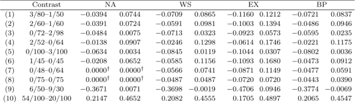
2

. Table 3.1 shows 95% limits of RD. The rows (1) and (2) represent no zero cells(NZ) with rare events, (3) to (6) depict one zero cell(OZ), and (7) and (8) are two zeros in the same row(RZ). (9) and (10) are general cases having moderate numbers. As shown in (9) and (10), if the number of events is moderate, all methods are similar although there are diﬀerences in size; the CI of the exact method are very broad while the Wilson score method and the Bayesian probability method are relatively narrow. The results are quite diﬀerent when events are rare.

Especially, when both events are zero, x

1

= 0 and x

2

= 0, the normal approximation method cannot calculate limits due inappropriate tethering.

Table 3.2 shows examples of RR. Rows (1) to (4) represent no zero cells(NZ) with rare events, (5)

to (8) are one zero cell(OZ), and (9) and (10) are results on a general setting like in the Table

3.1. Fieller-like method seems to have a problem when events occur rarely. Most of its lower limits

(7)

Table 3.1. 95% confidence intervals of RD for selected contrasts

Contrast NA WS EX BP

(1) 3/80–1/50 −0.0394 0.0744 −0.0709 0.0865 −0.1160 0.1212 −0.0721 0.0837 (2) 2/60–1/60 −0.0391 0.0724 −0.0591 0.0981 −0.1003 0.1394 −0.0486 0.0946 (3) 0/72–2/98 −0.0484 0.0075 −0.0713 0.0323 −0.0923 0.0573 −0.0595 0.0235 (4) 2/52–0/64 −0.0138 0.0907 −0.0246 0.1298 −0.0614 0.1746 −0.0221 0.1175 (5) 0/100–3/100 −0.0634 0.0034 −0.0845 0.0119 −0.1044 0.0307 −0.0802 0.0036 (6) 1/45–0/45 −0.0208 0.0652 −0.0585 0.1156 −0.1093 0.1680 −0.0473 0.0912 (7) 0/48–0/64 0.0000^† 0.0000^† −0.0566 0.0741 −0.0871 0.1149 −0.0477 0.0591 (8) 0/75–0/75 0.0000^† 0.0000^† −0.0487 0.0487 −0.0720 0.0720 −0.0443 0.0390 (9) 6/50–9/30 −0.3671 0.0071 −0.3698 −0.0019 −0.4706 0.0946 −0.3774 −0.0069 (10) 54/100–20/100 0.2147 0.4652 0.2082 0.4555 0.1705 0.4897 0.2065 0.4547

†: inappropriate tethering

Table 3.2. 95% confidence intervals of RR for selected contrasts

Contrast NA FL LB BP

(1) (1/10)/(2/20) 0.1025 9.7504 < 0.0000^§ 0.1694 0.1335 6.9106 0.1574 6.2672 (2) (3/80)/(1/50) 0.2005 17.5327 < 0.0000^§ 0.4728 0.2763 13.0177 0.2695 9.7889 (3) (1/20)/(1/20) 0.0670 14.9046 < 0.0000^§ 0.1603 0.1064 9.3925 0.1083 7.5447 (4) (1/200)/(2/200) 0.0629 15.8777 < 0.0000^§ 0.1590 0.1046 9.5594 0.1098 9.5692 (5) (0/72)/(2/98) 0.0000^† 0.0000^† < 0.0000^§ 0.0000 0.0000^† 0.0000^† 0.0133^‡ 3.5753 (6) (0/10)/(2/15) 0.0000^† 0.0000^† < 0.0000^§ 0.0000 0.0000^† 0.0000^† 0.0124^‡ 2.9579 (7) (0/100)/(3/100) 0.0000^† 0.0000^† < 0.0000^§ 0.0000 0.0000^† 0.0000^† 0.0084^‡ 1.6148 (8) (0/20)/(1/20) 0.0000^† 0.0000^† < 0.0000^§ 0.0000 0.0000^† 0.0000^† 0.0119^‡ 5.0990 (9) (6/50)/(9/30) 0.1580 1.0123 0.1737 1.1836 0.1613 0.9894 0.1734 0.9833 (10) (54/100)/(20/100) 1.7533 4.1577 1.8382 4.4822 1.7786 4.1951 1.8004 4.1806

†: inappropriate tethering, §: overt overshooting, ‡: point estimate out of limits

show overt overshooting. OZ show inappropriate tethering for normal approximation method and likelihood based method. However, all Bayesian probability methods have both lower and upper limits although its point estimate is out of estimated interval limits. We discuss this more in detail in the last section.

As shown in the examples, neither RD nor RR has any problem for all methods with a moderate number of events. Only a rare event causes problems, which implies we have to choose a method with caution when handling rare events. We examine eight methods for RD and RR in the next section through Monte-Carlo simulations.

4. Simulations

We present the results of the Monte-Carlo simulation to compare the performances of the afore-

mentioned interval estimates of RD and RR when the probability of the disease is small. For RD,

we employed the study design used by Newcombe (1998b). Let θ = p

1

− p

2

be a parameter of

interest and ψ = (π

1

+ π

2

)/2 be a nuisance parameter. 10, 240 parameter space points are chosen

from sample sizes m = 50, 60, . . . , 200, n = 50, 60, . . . , 200. For each (m, n) pair, 40 (ψ, θ) pairs

are generated randomly by θ = λ{0.1 − |2ψ − 0.1|} and ψ ∼ U(0, 0.1) and λ ∼ U(0, 1) so that

0 ≤ p

1

≤ 0.1 and 0 ≤ p

2

≤ 0.1 are maintained. A total of 10,000 samples are generated in each set

of the parameter (ψ, θ). For RR, we used the same design as the RD except that we generated p

1

(8)

Table 4.1. Estimated coverage probabilities for 90%, 95%, and 99% CI of RD

Method 90 % coverage 95% coverage 99% coverage

Min. Mean Max. Min. Mean Max. Min. Mean Max.

NA 0.1202 0.1204 0.8951 0.9597 0.85148 0.9196 0.1204 0.93349 0.9938 WS 0.8681 0.9395 0.9693 1.0000 0.92657 1.0000 0.9888 0.99604 1.0000 EX 0.2285 0.9755 0.99469 1.0000 0.84842 1.0000 0.9953 0.99913 1.0000 BP 0.8145 0.9169 0.9615 1.0000 0.91897 1.0000 0.9827 0.99261 1.0000

Table 4.2. Estimated average CI size of RD

Method 90% 95% 99%

NA 0.08773 0.10452 0.13732

WS 0.10045 0.12429 0.17565

EX 0.11093 0.13410 0.17937

BP 0.09724 0.11755 0.15954

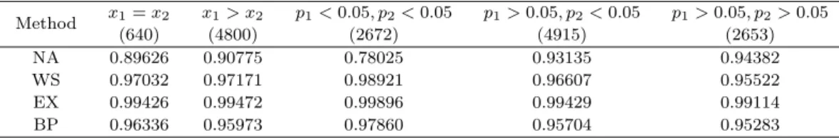
Table 4.3. Estimated coverage probabilities for 95% CI of RD for parameter space points(number of sample points) Method x1= x2 x1> x2 p1< 0.05, p2< 0.05 p1> 0.05, p2< 0.05 p1> 0.05, p2> 0.05

(640) (4800) (2672) (4915) (2653)

NA 0.89626 0.90775 0.78025 0.93135 0.94382

WS 0.97032 0.97171 0.98921 0.96607 0.95522

EX 0.99426 0.99472 0.99896 0.99429 0.99114

BP 0.96336 0.95973 0.97860 0.95704 0.95283

and p

2

from U (0, 0.1) and U (0, 0.1) respectively for simplicity.

To evaluate performances, we measure the coverage probability of interval estimates and compare with the nominal level. Coverage probabilities are compared diﬀerently depending on the observed proportions and the sample sizes.

In the Bayesian probability method, independent uniform distributions are used as the prior distributions of p

1

and p

2

to represent prior ignorance. Then, a posteriori p

1

and p

2

are independent beta distributions with parameters (x

1

+ 1, n

1

− x

1

+ 1) and (x

2

+ 1, n

2

− x

2

+ 1) respectively.

4.1. Risk diﬀerence

Table 4.1 displays the estimated coverage probabilities under 95%, 90%, and 99% of the nominal

conﬁdence levels. All but the normal approximation method(NA) maintain nominal levels. The

mean of the coverage probabilities of the Wilson score method(WS) was similar to the Bayesian

probability method(BP) but the BP has a shorter range than the WS. The NA cannot be compared

with others because of the tethering problem. The BP results in the most narrow CIs, while the

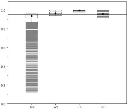
Exact method(EX) is most conservative. Figure 4.1 shows box plots of 95% coverage probabilities

of the four methods. The horizontal line in the ﬁgure shows 95% nominal level. NA had many

outliers; however, other methods resulted in short ranges. BP and WS are close to the nominal

level; EX is more conservative than the others are. When we divided the results by subsets of

parameters, as shown in Table 4.3, BP shows very stable coverage probabilities, however, EX and

WS show higher coverage probabilities than the nominal level except when both proportions are

larger than 0.05 as in the last column. In addition, NA shows lower than the nominal level except

when both proportions are larger than 0.05.

(9)

0.0 0.2 0.4 0.6 0.8 1.0

NA WS EX BP

Figure 4.1. Box-plots of 95% coverage probabilities for RD

Table 4.4. Estimated coverage probabilities for 95%,90%,and 99% CI of RR

Method 90% coverage 95% coverage 99% coverage

NA 0.0000 0.83016 0.9388 0.0000 0.87153 0.9775 0.0086 0.89986 0.9990 FL 0.0000 0.69528 0.9309 0.0000 0.63935 0.9570 0.0000 0.46511 0.9860 LB 0.0000 0.81810 0.9184 0.0000 0.86080 0.9601 0.0000 0.89502 0.9941 BP 0.7342 0.90360 0.9308 0.8532 0.95093 0.9680 0.9364 0.98931 0.9949

4.2. Risk ratio

Table 4.4 shows the coverage probabilities for the 95%, 90%, and 99% nominal levels. Since in many

cases the simulation resulted in where RR cannot be deﬁned, we treat undeﬁned case as zero point

estimates and zero size. Normal approximation(NA), Fieller-like method(FL), and likelihood based

method(LB) show zero minimum coverage because we treated and undeﬁned case as zero and have

wide ranges accordingly, whereas the Bayesian probability method(BP) is very stable throughout

the range and maintains the nominal level in mean coverage. Table 4.5 shows a very large average

size for the BP; however, it does not perform badly because others show a small average CI size due

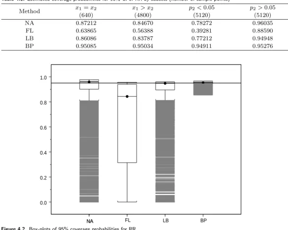
to tethering or overt overshooting. Figure 4.2 represents box plots for the four methods. All are

skewed and have outliers shown as shaded parts in the ﬁgure. For FL, the box extends for almost

the whole range and outliers are truncated by the zero value. Further, mean coverage probabilities

of FL in Table 4.4 are lower than the nominal levels. In addition to the fact that limits do not exist

for x

1

and/or x

2

= 0, FL appears uncommon limits when z

α/2

is large or when ˆ p

2

is small. For

rare events, BP performs well while others perform badly.

(10)

Table 4.5. Estimated average length of RR

Method 90% 95% 99%

NA 9.3393 12.6148 22.245

FL 31.9641 38.6972 95.166

LB 7.8933 10.1417 15.350

BP 26.5618 50.2463 227.614

Table 4.6. Estimated coverage probabilities for 95% CI of RR by subsets (number of sample points)

Method x1= x2 x1> x2 p2< 0.05 p2> 0.05

(640) (4800) (5120) (5120)

NA 0.87212 0.84670 0.78272 0.96035

FL 0.63865 0.56388 0.39281 0.88590

LB 0.86086 0.83787 0.77212 0.94948

BP 0.95085 0.95034 0.94911 0.95276

0.0 0.2 0.4 0.6 0.8 1.0

NA

NA FL LB BP

Figure 4.2. Box-plots of 95% coverage probabilities for RR

Table 4.6 shows performances by subsets. We divided subset of parameters only by p

2

because the proportion of denominator is more sensitive to the results. However, regardless of subsets, the results are similar to those in Table 4.4. The results are improved when p

2

is greater than 0.05.

5. Discussion

We performed Monte Carlo simulations to evaluate various interval estimates of RD and RR when

the probability of the disease to occur is small and when it is proposed for use with the Bayesian

probability method. Our simulation results showed that the Wilson score method, the exact method,

and the Bayesian probability method work well for RD and the normal approximation method, the

likelihood based method, and the Bayesian probability method perform well for RR.

(11)

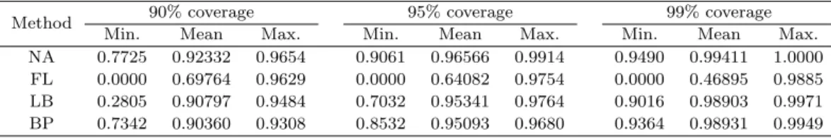
Table 5.1. Estimated coverage probabilities of RR by adding 0.5 for ZERO case

Method 90% coverage 95% coverage 99% coverage

NA 0.7725 0.92332 0.9654 0.9061 0.96566 0.9914 0.9490 0.99411 1.0000 FL 0.0000 0.69764 0.9629 0.0000 0.64082 0.9754 0.0000 0.46895 0.9885 LB 0.2805 0.90797 0.9484 0.7032 0.95341 0.9764 0.9016 0.98903 0.9971 BP 0.7342 0.90360 0.9308 0.8532 0.95093 0.9680 0.9364 0.98931 0.9949

Table 5.2. Estimated average CI size of RR by adding 0.5 for ZERO case

Method 90% 95% 99%

NA 30.0145 45.3518 101.972

FL 15.5881 16.4862 59.787

LB 22.2492 29.2557 45.986

BP 26.5618 50.2463 227.614

The normal approximation method of RD should be avoided when the probability of the disease to occur is small. The exact method is very conservative even when the nuisance parameter is eliminated on a restricted range. The Wilson score method performed well along with the Bayesian probability method, but it is more conservative than the Bayesian probability method. In the RR results, only Bayesian is recommended for inference of RR with rare events.

Regarding aberrations, we showed some examples of tethering and overt overshooting and examined them. The normal approximation method shows tethering for RD and Fieller-like method has many overt overshootings for RR. The Bayesian probability method for RR has an aberration resulting in some point estimates are out of estimated interval limits. The Bayesian probability method is adjusted by prior distribution. It can be used in zero event situations by adding 0.5 effect for absent cases. Four methods are compared in Table 5.1 and Table 5.2 for RR only. The tables show coverage probabilities and mean CI sizes when 0.5 is added for absent event. The results for the Bayesian probability method is the same as in the Table 4.4 and Table 4.5. The normal approximation method and the likelihood based method are improved. In contrast, the Fieller-like method does not improve by adding 0.5. The results of the likelihood based method are comparable to those of the Bayesian probability method in the coverage probabilities; however, the likelihood based method is not time-efficient because of iterative way to find limits

The Bayesian probability method showed very good performance for both RD and RR. It does not depend on the balance of sizes between two samples and on the variety in true values of the parameter. Besides the coverage probabilities and interval size, computational simplicity is an im- portant factor in the evaluation of interval estimates. From the computational point of view, we recommend the Bayesian probability method since the calculation of the Bayesian probability intervals only requires random number generation that can be easily done with standard software and the interval estimates of RD and RR can be constructed simultaneously using the same generated random numbers.

References

Aitchison, J. and Bacon-Shone, J. (1981). Bayesian risk ratio analysis, The American Statistician, 35, 254–257.

Bickel, P. J. and Doksum, K. A. (1977). Mathematical Statistics: Basic Ideas and Selected Topics, Holden- Day.

(12)

Beal, S. L. (1987). Asymptotic conﬁdence intervals for the diﬀerence between two binomial parameters for use with small samples, Biometrics, 43, 941–950.

Berger, R. L. and Boos, D. D. (1994). P Values maximized over a conﬁdence set for the nuisance parameter, Journal of the American Statistical Association, 89, 1012–1016.

Chan, Ivan S. F. (1998). Exact tests of equivalence and eﬃcacy with a non-zero lower bound for comparative studies, Statistics in Medicine, 17, 1403–1413.

Ewell, M. (1996). Comparison methods for calculating conﬁdence intervals for vaccine eﬃcacy, Statistics in Medicine, 15, 2379–2392.

Gart, J. J. and Nam, J. M. (1988). Approximate interval estimation of the ratio of binomial parameters: A review and corrections for skewness, Biometrics, 44, 323–338.

Gelman, A., Carlin, J. B., Stern, H. S. and Rubin, D. B. (1995). Bayesian Data Analysis, Chapman & Hall.

Katz, D., Baptista, J., Azen, S. P. and Pike, M. C. (1978). Obtaining conﬁdence intervals for the risk ratio in cohort studies, Biometrics, 34, 469–474.

Koopman, P. A. R. (1984). Conﬁdence limits for the ratio of two binomial proportions, Biometrics, 40, 513–517.

Louis, T. A. (1981). Conﬁdence intervals for a binomial parameter after observing no successes, The Amer- ican Statistician, 35, 154–154.

Mee, R. W. (1984). Conﬁdence bounds for the diﬀerence between two probabilities, Biometrics, 40, 1175–

1176.

Miettinen, O. S. and Nurminen, M. (1985). Comparative analysis of two rates, Statistics in Medicine, 4, 213–226.

Newcombe, R. G. (1998a). Two-sided conﬁdence intervals for the single proportion: Comparison of seven methods, Statistics in Medicine, 17, 857–872.

Newcombe, R. G. (1998b). Interval estimation for the diﬀerence between independent proportions: Com- parison of eleven methods, Statistics in Medicine, 17, 873–890.

Noether, G. E. (1957). Two conﬁdence intervals for the ratio of two probabilities and some measures of eﬀectiveness, Journal of the American Statistics Association, 52, 36–45.

Santner, T. S. and Snell, M. K. (1980). Small-sample conﬁdence intervals for p1− p2 and p1/p2 in 2× 2 contingency tables, Journal of the American Statistical Association, 75, 386–394.

Walter, S. D. (1975). The distribution of Levin’s measure of attributable risk, Biometrika, 62, 371–375.

Wilson, E. B. (1927). Probable inference, the law of succession, and statistical inference, Journal of the American Statistical Association, 22, 209–212.