1. Introduction
1)
High precision population distribution data are extremely important in numerous decision making and real world problem solving efforts. Examples include those in business, healthcare, national security, and emergency response and preparedness applications(Dobson et al. 2003; Hay et al. 2005;
Langford and Higgs 2006; Garb et al. 2007).
Population estimation often boils down to the redistribution of spatially aggregated census count data to spatial units of finer resolution a – process of spatial interpolation. In other words, population interpolation refers to the process of transferring population data from one set of spatial units (source zones) to another (target
**This work was supported by the National Research Foundation of Korea Grant funded by the Korean Government(NRF-2013S1A5A8023119)
**Assistant Professor, Department of Geography, Chonnam National University([email protected])
Locally adaptive intelligent interpolation for population distribution modeling using pre-classified land cover
data and geographically weighted regression *
Hwahwan Kim **
지표피복 데이터와 지리가중회귀모형을 이용한 인구분포 추정에 관한 연구*
김 화 환 **
Abstract:Intelligent interpolation methods such as dasymetric mapping are considered to be the best way to disaggregate zone-based population data by observing and utilizing the internal variation within each source zone.
This research reviews the advantages and problems of the dasymetric mapping method, and presents a geographically weighted regression (GWR) based method to take into consideration the spatial heterogeneity of population density - land cover relationship. The locally adaptive intelligent interpolation method is able to make use of readily available ancillary information in the public domain without the need for additional data processing.
In the case study, we use the preclassified National Land Cover Dataset 2011 to test the performance of the proposed method (i.e. the GWR-based multi-class dasymetric method) compared to four other popular population estimation methods (i.e. areal weighting interpolation, pycnophylactic interpolation, binary dasymetric method, and globally fitted ordinary least squares (OLS) based multi-class dasymetric method). The GWR-based multi-class dasymetric method outperforms all other methods. It is attributed to the fact that spatial heterogeneity is accounted for in the process of determining density parameters for land cover classes.
Key Words:population estimation, spatial interpolation, dasymetric mapping, spatial heterogeneity, geographically weighted regression(GWR), National Land Cover Dataset(NLCD).
요약 데시메트릭 매핑은 행정구역 단위로 집계된 인구자료를 행정구역 내부의 공간적 변이에 따라 재집계하여 고해: 상도의 인구분포 자료를 작성하는 가장 보편적인 기법이다 본 연구에서는 데시메트릭 매핑을 이용한 인구분포 추정. 의 장단점을 검토하고 그 개선방안으로서 지리가중회귀모형을 이용한 다변량 데시메트릭 매핑 기법을 제안하였다 기, . 존의 지표피복 데이터와 인구센서스 자료를 기반으로 지리가중회귀모형을 적용하여 각 집계단위별로 지표피복 유형과 인구밀도의 상관관계를 분석하고 모형에서 산출된 회귀계수를 이용해 하위 공간구획의 인구 총수를 산정하였다 그 , . 결과 지리가중회귀모형 기반 다변량 데시메트릭 매핑 기법을 이용했을 때 면적가중 보간법 이진 데시메트릭 매핑, , , 피크노필렉틱 보간법 최소자승회귀모형 기반 데시메트릭 매핑 기법 등 다른 지능형 보간법에 비해 정확한 인구분포 , 추정이 가능하다는 것을 확인하였다 이는 지리가중회귀모형을 통해서 인구센서스 집계 단위별로 상이한 구역 내 공. 간적 이질성이 인구분포 추정에 적절히 반영되었기 때문인 것으로 평가할 수 있다.
주요어 인구분포 추정 공간보간법 데시메트릭 매핑 공간적 이질성 지리가중회귀모형: , , , , , NLCD
zones). The literature is replete with various population estimation methods using spatial interpolation. According to the type of information in use, we can classify population interpolation methods into two types, those based on spatial configuration only, and those that employ not only spatial configuration but also additional ancillary information such as spatial distribution of land use and land cover types(Wu et al. 2005).
The first type uses no additional information besides the sets of spatial units and the population counts in the source zones. Examples include the areal weighting interpolation(Goodchild and Lam 1980), pycnophylactic interpolation(Tobler 1979), and kernel-based interpolation(Martin 1989).
The second type of population interpolation employs not only the above information, but also so-called ancillary information with the purpose to integrate internal variations of source zone.
The second type of methods are also called
‘intelligent’ interpolation methods by some researchers(Flowerdew and Green 1994). Dasymetric mapping method is the most typical, if not the only, example of those intelligent interpolation methods. It has been increasingly popular, especially due to the rapidly growing availability of geographic data and increasing popularity of geographic information system (GIS) and remote sensing (RS) technologies.
Many studies have demonstrated that the dasymetric method can substantially improve population estimation accuracy(Mrozinski and Cromley 1999; Reibel and Agrawal 2007; Langford 2006). In fact, some earlier comparative studies concluded that dasymetric mapping was the best performer among all popular population interpolation methods(Fisher and Langford 1995;
Cockings et al. 1997; Mrozinski and Cromley 1999). Despite the significant performance advantages of the dasymetric mapping, there has been little evidence to suggest widespread adoption amongst the broader GIS community(Langford
2007). Langford(2007) stated that intelligent methods were not widely adopted because of two reasons. First, implementation of intelligent interpolation is much more complicated than simple areal weighting interpolation which can be implemented by a suitable overlay tool which is readily available in most GIS software.
Furthermore, most intelligent interpolation methods require additional process to prepare ancillary information. For instance, many researchers had to perform land use land cover classification with satellite images to obtain ancillary data for intelligent interpolation of population(Langford and Unwin 1994; Yuan et al. 1997; Holt et al.
2004; Reibel and Agrawal 2007; Sleeter 2004).
Areal weighting interpolation does not require the user to be involved with the preparation of ancillary data. Moreover, these additional processes may also introduce more errors into the original dataset because the accuracy of those ancillary data is not assured and errors are inherent in almost all aspects of GIS analysis. Therefore, there is no wonder that many users still prefer the traditional simple interpolation method despite the superior performance by the intelligent interpolation methods reported in many studies. To encourage the geography community to employ intelligent interpolation methods, efforts should be made to overcome the problems of excessive processing time and implementation difficulty. Regarding the acquisition of high accuracy ancillary information, there are several high quality public-domain datasets available in the United States such as the National Land Cover Dataset(NLCD). The NLCD data are free, seamless, and intended to be updated regularly, which is vital for timely estimation. Making use of the readily available ancillary data not only guarantees the currency of data, but also helps to minimize the data processing time.
Another problem with the dasymetric mapping
and other ‘intelligent’ population interpolation
methods is that they ignore spatial heterogeneity (or non-stationarity) in the relationship between population distribution and the distribution of explanatory variables(e.g., land use land cover classes). Although the current methods account for the spatial heterogeneity of population density within each source zone by incorporating, for instance, land use land cover ancillary information, it assumes that the relationship between the population density and any specific land use land cover type is spatially stationary. Such relationship, in reality, varies across space. For instance, it is likely that a range of residential densities are present within most census reporting zones even though the corresponding land use land cover types are the same(Langford 2006).
The difference in residential densities arises primarily due to different housing types in the urban areas. That is, the population density of a residential area in the city center is highly probable to be different from that of a suburban town. This problem has been realized by many researchers who make use of the ordinary least squares (OLS) regression model in population estimation. Some attempts have been made to deal with this problem by adopting regional regression approaches, in which the whole study area is subdivided into smaller regions and an OLS regression model is applied to each region to estimate the population. Such an approach seems to produce better results for each region (Langford 2006; Yuan et al. 1997). Albeit a good try, such a solution has obvious flaws. First, it is difficult to know how large or small a region should be. Therefore there is no guarantee of sufficient account of spatial heterogeneity in a study. Secondly, repeating the same process over multiple regions in one study is tedious and deficient.
This research responds to both of the above discussed problems of intelligent interpolation method by introducing the geographically
weighted regression(GWR). The GWR method has been designed specifically to take care of the spatial heterogeneity problem(Fotheringham et al.
2002). We present a GWR-based intelligent interpolation method with a two-fold objective.
On one hand, the method is anticipated to effectively account for the spatial heterogeneity of relationships between population density and ancillary information. On the other hand, the method is designed in order to allow users to directly make use of readily available multi-class land use land cover data. The remainder of the article is organized as follows. The next section examines the existing theoretical framework relating to population interpolation methods and to the issue of spatial heterogeneity. Section 3 presents the GWR-based intelligent interpolation method with a case study. The article concludes in Section 4 with a summary of findings and discussions of future work.
2. Areal Interpolation Methods for Population Estimation
Cross-area estimation or areal interpolation is primarily designed for transferring data between two sets of non-nesting spatial units (Goodchild and Lam 1980). The two spatially incompatible zoning units are usually termed source zone and target zone.
1) Areal weighting interpolation
The simplest areal interpolation technique is
areal weighting interpolation. The methodology is
based only on the geometric intersection of the
source and target zones. It assumes homogeneity
within source zones and therefore no further
ancillary information is required to guide the
interpolation process. Population of each target
zone is estimated by the following equation
(Fisher and Langford 1995):
å
==S ´
s s
s ts
t A
P P A
1
ˆ (1)
where, S is the number of source zones;
is the area of overlap between target zone t and source zone s;
is the population of source zone s; and
is the area of source zone s. The problem with this method is the unfounded assumption of uniform spatial distribution of population density within each source zone.
Numerous studies have shown the overall low accuracy of simple area weighting in comparison to other techniques, e.g., intelligent interpolation (see for example, Langford 2006; Gregory 2002;
Reibel and Agrawal 2007; Mrozinski and Cromley 1999; Sadahiro 2000)
2) Pycnophylactic interpolation
Pycnophylactic interpolation denies the assum- ption of homogeneity of population density within source zones. Tobler (1979) proposed this method for the preparation of a smoothed map (or isopleth map) from data in discrete areal spatial unit system, assuming the existence of a smooth density function which is non-negative and has a finite value for every location. The virtue of this interpolation method is to redistribute source zone values by distance-decay density function while ensuring original value in the source zone intact the so called pycnophylactic or volume - – preserving property. This property can be defined in equation(2), according to Lam(1983).
å
=ij ij k k
ijq p
az ,
å
=ij ij k
k A
aq , and
å
=k kij
q 1
(2)
Where,
is the original population of zone
,
is the area of zone
,
is the density in cell
, and
is the area of each cell.
is set
to 1 if
is in zone
; otherwise set it at 0.
The interpolation procedure begins by assigning the mean density to each grid cell superimposed on the source zones, and then modifies the assigned values by slight amounts to bring the density closer to the value required by the governing partial differential equation(Tobler, 1979).
òò
=Ri
Hi
dxdy y x Z( , )
(3)
Where,
denotes the
region and
is the total population count in region
. The volume- preserving condition is then enforced by either incrementing or decrementing all the density values within individual zone at the end of each iteration.
3) Dasymetric mapping method
Dasymetric mapping (DM) methods are typical
intelligent interpolation methods as they require
and make use of ancillary information to infer
internal structure of population distribution within
source zones. Dasymetric mapping, first developed as
a form of cartographic representation(McCleary
1984), is defined as a method by which source
zones are subdivided into cellular units that possess
greater internal consistency in the densities of the
variable being mapped. Often land use and land
cover types are used as ancillary information,
although other information such as building and
street has also been used. According the classification
scheme in the ancillary information, we can
classify DM methods into binary DM and
multi-class DM. The simplest is binary DM in
which a binary land use (or other ancillary data)
classification is used to control the population
allocation. A cellular unit is classified either as
residential (populated) or non-residential (non-
populated) type so that population can be
re-distributed to those residential units only(Fisher
and Langford 1995; Fisher and Langford 1996).
The method is different from the areal weighting interpolation as it only considers the populated areas in the target zones for allocating population.
It is conceptually simple and practically outperforms other non-intelligent methods(Eicher and Brewer 2001; Martin et al. 2000; Langford 2006, Langford 2007). However, there are two major limitations of the binary DM. First, it is unable to address more complex relationships between land uses and a variety of population concentration. In reality, a range of population densities are present within most census reporting zones by different land uses, particularly in urban areas(Langford 2006). Secondly, because such binary classification of residential versus non-residential land use classes is rarely available directly, this method often requires researchers and practitioners to invest considerable time in preparing such ancillary data.
The Multi-class DM is an incremental deve- lopment from the binary DM (e.g. see Langford 2006 for a summary). The most important issue of the multi-class DM is how to calibrate density parameters for different land cover classes. Unlike that in the binary DM where population density in ‘non-populated’ cellular units is fixed to zero and that in the ‘populated’ area is calibrated by a simple algebra as used by the areal weighting interpolation, the determination of densities for multiple classes in the multi-class DM is complicated. There are several ways reported in the literature to determine the population density for each class. These methods have been categorized into the following three groups (Langford 2006);
Proportion preset, Selective sampling, and Statistical modeling.
Proportion preset assigns a subjectively pre- defined proportion of the total population to each class(Eicher and Brewer 2001). Thus the density can be determined accordingly. Selective sampling determines population density parameters
by a selective sampling strategy. For example, the density for a class can be easily calculated by selecting a number of source zones filled by that single land cover class only(Mennis 2003), assuming enough samples can be found. But often it is difficult or simply not possible to find enough number of source zones filled by a single land cover class. In response, some other modified methods, such centroid sampling, containment sampling, and percent cover sampling, have been proposed to loosen the sampling requirement (Mennis and Hultgren 2006). Statistical modeling is a more generalized solution (Langford et al.
1991; Yuan et al. 1997; Langford 2006) using statistical modeling. It aims to establish a multivariate regression model to estimate the population in a zone to surrogate variables of multiple land use/land cover classes. The surrogate variable for each class is usually the number of cellular units of that class in the zone. In this case, the regression coefficient of this variable is the density of the corresponding class.
4) The spatial heterogeneity problem and intelligent population estimation
All of the previous solutions of multi-class
dasymetric mapping share a common limitation –
the lack of consideration of heterogeneity in the
relationship between the ancillary information
and population density. Heterogeneity refers to
the fact that, unlike physical laws, measurement
of social processes tends to vary according to
where it is made(Fotheringham 2002). In the case
of spatial processes, it is referred to as spatial
heterogeneity, or in other words, the relationship
measurements tend to vary over space. Research
by Langford (2006) revealed the presence of
spatial heterogeneity in the relationship between
population and land cover, which the global
regression models cannot handle. For population
estimation, the OLS regression model assumes
that there exists a spatially stationary relationship between population and land cover as there is only one set of coefficients applying to all areas.
However, this assumption is not problematic for the above discussed intelligent population estimation, particularly when the ancillary information is the classified land cover raster data which is widely available. In remote sensing classification, an important distinction is made between land use and land cover. Satellite images can reveal land cover such as man-made structures, water, bare soil, trees, and so on, through the unique spectral characteristics of each type. Thus land cover data is relatively easy to be classified and such classification is a standard function in most remote sensing software. Land uses, however, have to be interpreted based on the land cover information and many additional information such as shape, size, etc. Such interpretation requires specific expert skills and consequently involves certain level of subjectivity. In fact, different land uses could be conjectured from a single land cover dataset depending on the procedure that was used and who did the interpretation. This is the probably the major reason why land cover data are much more widely available than land use data. When we use this type of ancillary information for intelligent population estimation, the multi-class land cover data only show, for instance, if a piece of land is developed and how much it is developed (open, low, medium, and high intensity) but not directly the information about what land uses might be associated.
For example, high intensity developed pixels might be apartment complexes, row houses, and commercial/industrial without saying what exactly it is. It is highly probable that pixels with the same land cover class might have different land uses depending on where the pixel is located.
Hence, a density parameter for each land cover class might vary spatially. Furthermore, the land use land cover extracted from the satellite images
cannot be 100% accurate and spatial variability of classification errors occurs(Lo 2008). All these give rise to spatial heterogeneity, which the OLS model cannot address. The accuracy of a population land use model for population estimation – does not depend totally on the independent variables used or any other ancillary data included. It appears that a local rather than a global approach is needed to deal with the spatial heterogeneity of the input data in the model.
Such a problem has been realized by many researchers who make use of the OLS regression model in population estimation. Some attempts have been made to deal with this problem by adopting a regional regression approach, in which the whole study area is subdivided into smaller regions, and an OLS regression model is applied to each region to estimate the population. Such an approach is reported to produce better results for each region(Yuan et al. 1997; Huang and Leung 2002; Langford 2006). However, it is difficult to know how large a region should be.
Some previous studies use county as the unit of region(e.g. Yuan et al. 1997). The model still suffers from the same problem of spatial hetero- geneity as a county is large enough to contain spatial variations in itself.
Recently, there is an increased interest in the use of local geographically weighted regression (GWR) in human geography, which has been designed specifically to take care of the spatial heterogeneity problem(Fotheringham et al. 2002;
Huang and Leung 2002). GWR extends an ordinary least squares regression model by allowing local variations of coefficients(and thus relationships), as shown in Equation (4) (Lo 2008):
i n
k ik ik i
i a a x e
Y = +
å
+=1
0 i=1,2,……,n (4)
where,
and
are the dependent and
independent variables at point
;
=1, 2,...n,
and
are parameters to be estimated;
is the value of the
th parameter at location
; and
are independent normally distributed error terms with zero mean and constant variance at point
.
Unlike the OLS regression model which assumes global parameters across the whole study area, the GWR accounts for spatial variations by estimating local rather than global parameters for each individual observation. The GWR local coefficients can be estimated through a weighted least square procedure (see model calibration for estimation details).
3. GWR-based intelligent interpolation method for population estimation
This article presents a GWR-based intelligent population estimate method. By taking advantage of the recent developments in dealing with the
spatial heterogeneity problem and the increasingly availability of high quality national land cover data, the study aims to improve both the estimation accuracy and ease-of-use of the intelligent population methods. We will explain the method and evaluate its performance with a case study.
1) Data and study area
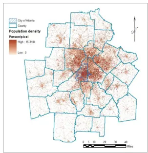
The Atlanta Metropolitan Statistical Area (MSA) is a rapidly changing area. The various types and stages of developments give rise to the spatial heterogeneity of spatial processes and relationships pertinent to population density. For the past decades, the region has been one of the fastest growing metropolises in the U.S. with a population increase of 39 percent during the period of 1990
2000(http://www.censusscope.org). <Figure 1>
–
shows the 28-county Atlanta MSA. The region has expanded greatly as suburbanization consumes large areas of forest and open land adjacent to
City of Atlanta Fulton
Meriwether Fulton Carroll
Cobb Bartow
Coweta
Jasper Henry
Pike Heard
Gwinnett
Walton Cherokee
DeKalb Paulding
Butts Newton Forsyth
Haralson
Pickens
Lamar Fayette
Dawson
Douglas
Spalding
Barrow
Clayton
Rockdale
Figure 1. Study area: Atlanta MSA, Georgia, USA.
(left: county boundaries, right: National Land Cover Dataset 2011)
the center city (city of Atlanta), pushing the peri- urban fringe farther away from the original urban boundary. Because of the significant physical growth, Atlanta’s urban spatial structure has changed dramatically(Yang and Lo 2002).
For population estimation, we use the 2010 census data for aggregated population counts and the NLCD 2011 for land cover ancillary information. Population counts at the census tract level for the 28-county Atlanta MSA were obtained from the U.S. Census Bureau. This dataset includes a total of 690 census tracts. At a finer level spatial granularity, census data in a total of 1,923 census block groups were also acquired for the purpose of accuracy evaluation.
A raster land cover dataset of the study area is extracted from the National Land Cover Dataset (NLCD) 2011, as displayed in the right-side map of <Figure 1>. The dataset is downloaded from the Multi-Resolution Land Characteristics Consortium (MRLC; http://www.mrlc.gov/). The NLCD 2011 dataset, derived from Landsat satellite images with a spatial resolution of 30m, provides pre-classified land cover information.
The NLCD program has many advantages for dasymetric mapping of population distribution.
Given that the difficulty of land cover classification is one of the main reasons why the dasymetric mapping method is not being widely accepted for population distribution mapping in spite of its better performance over simple areal weighting interpolation as briefly discussed above, a freely available land cover dataset like NLCD provides a good alternative to obtain land cover dataset for dasymetric mapping. Since the first distribution of NLCD in 1992, it was updated in 2001, 2006, 2011 respectively. It has been undertaken by MRLC since 2006 as a national land cover monitoring program. Regular update of the national land cover maps provides an opportunity for accurate population distribution mapping in timely manner.
The overall database philosophy and classifi- cation methodology were presented by Homer et al (2004; 2015). Particularly relevant to population estimation are the developed lands. The NLCD 2011 differentiates four types of developed land cover classes(i.e. high intensity, medium intensity, low intensity, and open space) according to the fraction of impervious surface, as summarized in
<Table 1>(Homer et al. 2015).
Code Class name Description
21 Developed, Open Space
Includes areas with a mixture of some constructed materials, but mostly vegetation in the form of lawn grasses. Impervious surfaces account for less than 20 percent of total cover. These areas most commonly include large-lot single-family housing units, parks, golf courses, and vegetation planted in developed settings for recreation, erosion control, or aesthetic purposes
22 Developed,Low Intensity
Includes areas with a mixture of constructed materials and vegetation. Impervious surfaces account for 20 49 percent of total cover. These areas most commonly – include single-family housing units.
23 Developed, Medium Intensity
Includes areas with a mixture of constructed materials and vegetation. Impervious surfaces account for 50 79 percent of the total cover. These areas most commonly – include single-family housing units.
24 Developed, High Intensity
Includes highly developed areas where people reside or work in high numbers.
Examples include apartment complexes, row houses, and commercial/industrial.
Impervious surfaces account for 80 to 100 percent of the total cover Table 1. NLCD 2011 classification scheme for developed land cover classes
2) Methodology
The proposed GWR-based multi-class dasymetric mapping method consists of a series of steps, most of which can be performed in a GIS software such as ESRI’s ArcGIS 10.1. The first task is to identify areas of populated land cover classes by source zones. It is to compute the proportion of grid cells in a source zone for each land cover class that might reasonably be expected to be inhabited. The four ‘developed’
land cover classes of the NLCD 2011 classification scheme are assumed to be inhabited and other land cover classes are excluded in further steps as no population counts need to be assigned to them. In the next step, the source zones’
population counts are then regressed on the calculated areas of the four populated (developed) land cover classes using the GWR model as expressed in Equation (4). The estimated model is then applied to each grid cell of the NLCD data layer so that a smoothed population density surface map can be generated. To evaluate the estimation accuracy, aggregated population counts at the block group level, which is finer than the census tract level, will be re-constructed from the population density surface map. The accuracy of the estimated block group level population counts can be calculated using the census data at the same level as the ground-truth data.
To assess the performance of the GWR-based method, we conducted population estimation with the same set of data using several other popular methods including areal weighting interpolation, binary dasymetric mapping, and traditional multi- class dasymetric methods using the OLS-based regression. Their performances are examined and compared.
3) Model calibration
Although all four types of models are calibrated
for the study area, we will explain calibration details for only the proposed methods because four other popular methods follow the same procedures as in the literature review. The GWR model provides locally varying parameter estimates for regression models where spatially varying relationships are hypothesized. We use the GWR 3.0 software which produces unique parameter estimates for all observations by spatially weighting the observations (i.e. census tract) according to their proximity to each other. Observations closer to each other are given more weight than are observations further away. The weights are derived through a distance-decay function to assign weights to data according to their proximity so that near locations have more influence than further locations. To limit the number of data points considered for each local parameter estimate, a spatial kernel is used at each observation. The kernel can be either fixed, in which case the bandwidth of the kernel is also fixed, and thus varying numbers of observations are weighted for the computation of each local parameter.
Because the census tracts in the Atlanta metro area have different sizes and are irregularly distributed, an adaptive kernel is more appropriate.
With an adaptive kernel, an equal number of data observations are weighted and used for local parameter estimation. In addition to local parameter estimates, the GWR program also provides local goodness-of-fit measures and local residuals. For this analysis, a geographically weighted Gaussian regression is applied to the whole study area at the census tract level using an adaptive kernel. The dependent variable is population count, and the four developed land cover classes are used as independent variables
<Table 2> shows a sample of input data, estimated parameters, local R
2, and residual of census tracts for the four-class GWR model.
The goodness-of-fit of the GWR model can
be assessed by examining several goodness-of-fit
measures of the model and those of the counterpart OLS model. <Table 3> shows such a comparison. Here the corresponding OLS model means it has the same dependent and independent variables as those of the GWR model. Both the Akaike Information Criterion (AIC) and the R
2measures indicate that the GWR model has clearly better goodness-of-fit than the OLS model does.
This suggests that explanation power of the regression modeling of population estimation can be greatly enhanced by accounting for local variations.
For high intensity developed land cover, the peripheral counties and parts of city center area exhibit the stronger positive relationship between high intensity developed land cover and population while most of the north-south belt of central counties shows a negative relationship(Fig. 2;
upper left map).
On the other hand, the local parameter estimates for the medium intensity developed land cover variable show high values (stronger
relationship) in the core and rapidly growing suburban counties(Gwinnett, Forsyth, and Barrow), gradually trending down to low values (weaker relationship) in the periphery(Fig. 2; upper right map). This displays a stronger core-periphery influence for Dev_med than that for the Dev_
high. As for the local parameter estimates for the low intensity developed land cover variable, which remain positive almost throughout(Fig. 2;
lower left map), the spatial distribution of the parameter estimates shows an inverse pattern from that of Dev_med. High population density areas such as the city core and major suburban residential area show weaker relationship between the area of Dev_low and population count while peripheral areas show stronger relationship. Finally, the local parameter estimates for the open-space developed land cover class interestingly show that a small ring of positive values (i.e., stronger relationship) in the city center(Fig. 2; lower right map). The most peripheral counties show negative values or weaker positive values, indicating weak
Goodness-of-fit measures Adjusted R2 AIC
GWR model 0.787 12,227
OLS model 0.657 12,436
Note : Higher adjusted R2 and lower AIC values indicate better goodness-of-fit
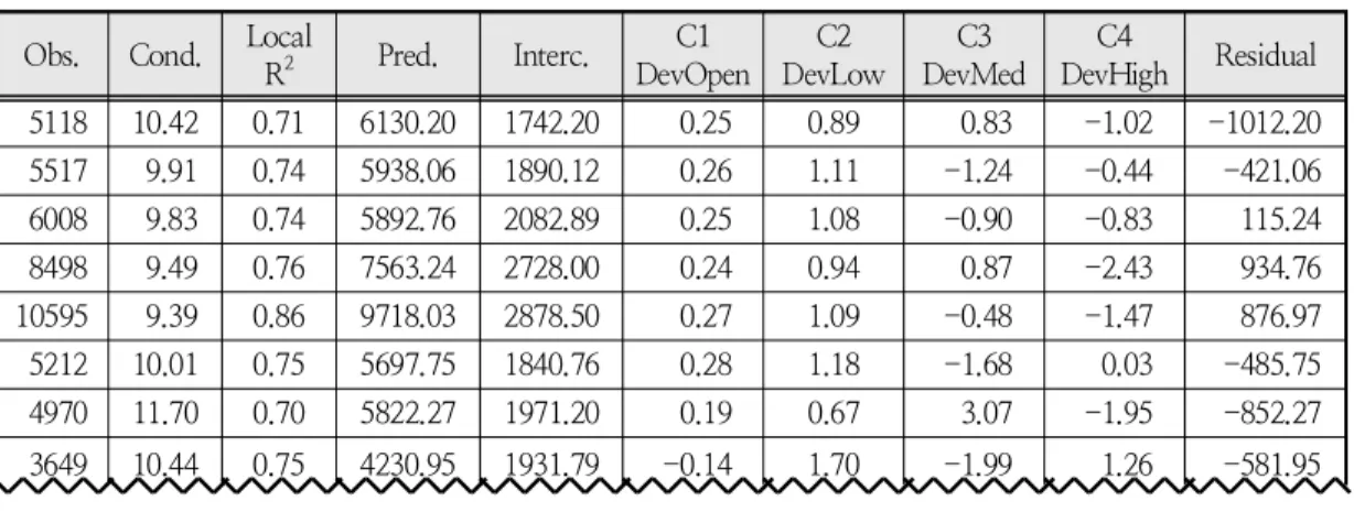
Table 3. Comparing the goodness-of-fit of the GWR and corresponding OLS models Obs. Cond. Local
R2 Pred. Interc. C1
DevOpen C2
DevLow C3
DevMed C4
DevHigh Residual 5118 10.42 0.71 6130.20 1742.20 0.25 0.89 0.83 -1.02 -1012.20 5517 9.91 0.74 5938.06 1890.12 0.26 1.11 -1.24 -0.44 -421.06 6008 9.83 0.74 5892.76 2082.89 0.25 1.08 -0.90 -0.83 115.24 8498 9.49 0.76 7563.24 2728.00 0.24 0.94 0.87 -2.43 934.76 10595 9.39 0.86 9718.03 2878.50 0.27 1.09 -0.48 -1.47 876.97 5212 10.01 0.75 5697.75 1840.76 0.28 1.18 -1.68 0.03 -485.75 4970 11.70 0.70 5822.27 1971.20 0.19 0.67 3.07 -1.95 -852.27 3649 10.44 0.75 4230.95 1931.79 -0.14 1.70 -1.99 1.26 -581.95
Table 2. Parameter estimation using the Four-class GWR model (sampled)
relationship between Dev_open and population.
The spatial pattern reveals a trend of values from low in the west to high in the east.
Taking the four-class model as a whole, the map of pseudo local
values shows the strongest relationship between population and land cover in some clusters south of the central city and most of peripheral areas. The weakest relationship is found in high density urban areas of Fulton, Cobb, DeKalb, and Clayton County around the central city (less than 0.5) (Fig. 3). This suggests that each of these parts has more complicated
residential density pattern, which is difficult to be modeled by only land cover areas.
Overall, the results of GWR model and the spatial pattern of parameter estimates for each land cover class show that spatial heterogeneity problem is evident in the relationship between land cover classes and population counts.
4) Implementation and performance evaluation Once the GWR and other popular population estimation models are calibrated, each model is
Figure 2. Distribution of regression coefficient values for the four ‘developed’ land cover classes.Dev_high (upper left), Dev_med (upper right), Dev_low (lower left), and Dev_open (lower right)
applied to the NLCD data layer to generate population density surface map. For the GWR- based model, it is important to recall, however, because the model does not accounts for all the variation in the source zone population, the density weights need to be locally scaled by the ratio of their respective source zone’s observed population to its fitted population to account for the proportion of source zone population not predicted in the model, thus preserving the pycnophylactic property (Flowerdew and Green 1989; Flowerdew and Green 1992; Yuan et al.
1997). For OLS regression model, where intercept and negative coefficient are excluded assuming no population for no residential area, the grid cells forming the raw estimated population surface were multiplied by the ratio of their respective source tracts’ observed populations to the source tract’s fitted population computed by summing the raw estimates across the source tract’s grid cells.
On the contrary, the GWR model does not exclude intercept term and negative parameter estimates provided that land cover class does not directly associated with residential land use.
Hence, we assume that a certain land cover may
have a negative effect on population density and intercept term could be a part of variance not explained by the four land cover class variables.
Assuming that the intercept term and error term in the GWR model refer to the variance that is not explained by the four developed land cover classes, those values are evenly redistributed to all developed pixels in each source zone. The result is the scaled population density surface map as shown in <Figure 4>. It is however noteworthy that the use of regression-based weights and pycnophylactic scaling is a practical solution that is not statistically valid.
In order to evaluate the performance of the proposed GWR-based population estimation model, several other popular independently implemented with the same data. <Table 4> lists the accuracy of estimated population at the block group level of each method, with the census block group population as ground-truth data. These Overall accuracy is assessed using mean absolute error (Goodchild et al. 1993) and root mean squared error (Eicher and Brewer 2001).
Several findings are revealed in <Table 4>. First
Figure 3. Local R2 valuesFigure 4. Population density surface from GWR based multi-class dasymetric method
of all, there is a clear distinction between the performance of intelligent interpolation methods and that of the simple interpolation methods.
The intelligent interpolation methods deliver much higher accuracy. The overall accuracy of binary dasymetric method is better than that of the multi-class dasymetric method based on the global regression model. This result is consistent with the previous finding of Fisher and Langford (1995). It suggests that, using a global regression model, benefits of additional information from multiple land cover classes rather than the binary land cover classes cannot be realized. It might be because of the ambiguity in the relationship between land cover and land use as discussed above. Finally and most importantly, the GWR- based intelligent interpolation outperforms all other methods. This method allows the spatial heterogeneity of land cover population density – correlation to be accounted for. GWR based dasymetric mapping allows any land cover class to have a negative density parameter as well as a positive parameter. Therefore, each land cover class may have varying density parameters area by area as shown in <Figure 2>, and <Table 2>.
Those figures show that a certain land cover class may have a negative effect on the population density in some regions, while positively correlated with population density in most areas, and vice versa. For instance, high intensity developed land cover has positive density parameters in the
eastern and western parts rural area while most of study area have negative parameters. On the other hand, medium intensity developed land cover shows negative parameters for those rural areas while positive parameters are prevalent in most areas.
4. Discussion and conclusion
This article examined the benefits of the geographical weighted regression (GWR) for dasymetric density parameter estimation in the context of population distribution modeling. For ancillary dataset used in the dasymetric method, we used the pre-classified NLCD 2011 land cover dataset that does not require digital image processing and classification. The performance of the GWR based multi-class dasymetric mapping method was examined by a comparative accuracy assessment with four other areal interpolation methods for population distribution modeling. All intelligent interpolation methods outperformed the areal weighting interpolation and the pycno- phylactic interpolation, both of which do not utilized ancillary information. OLS based multi- class dasymetric method did not show better performance than the binary dasymetric method.
GWR based multi-class dasymetric method was found to provide the most accurate result. The degree to which this technique was found to be superior is attributed to the fact that spatial
Method Mean absolute error (%) RMS error
Simple interpolation Areal weighting 37.21 941
Pycnophylactic 35.14 916
Intelligent interpolation
Binary dasymetric 26.58 769
Multi-class dasymetric
OLS regression 27.22 771
GWR 21.12 693
Note: total target zones N=1923, mean population of target zones = 6,156 Table 4. Performance summary
heterogeneity was accounted for in the process of determining density parameters for land cover classes.
Overall, this research showed that the perfor- mance of dasymetric mapping method can be improved by integrating the geographically weighted regression model to determine weight parameters of land cover classes on population density, which is a crucial part of the estimation process. It is also noteworthy that the proposed method performed well with the NLCD 2011, a publically available high quality national land cover dataset. We anticipate these data and methods would fulfill the need for accurate population distribution data without the effort to classify remotely sensed images.
References
Cockings, S., P. F. Fisher, and M. Langford.
1997. Parameterization and Visualization of the Errors in Areal Interpolation. Geographical Analysis 29 (4):314-328.
Dobson, J. E., E. A. Bright, P. R. Coleman, and B. L. Bhaduri. 2003. LandScan: A global population database for estimating population at risk. In Remotely Sensed Cities, edited by V. Mesev. London: Taylor & Francis.
Eicher, C., and C. Brewer. 2001. Dasymetric mapping and areal interpolation: implementation and evaluation. Cartography and Geographic Information Science 28:125-138.
Fisher, P. F., and Mitchel Langford. 1996.
Modeling sensitivity to accuracy in classified imagery: A study of areal interpolation. Profe- ssional Geographer 48 (3):299-309.
Fisher, Peter F., and M. Langford. 1995.
Modelling the errors in areal interpolation between zonal systems by Monte Carlo Simulation. Environment & Planning A 27:
211-224.
Flowerdew, R., and M. Green. 1989. Statistical
methods for inference between incompatible zonal systems. In The Accuracy of Spatial Databases, edited by M. F. Goodchild and S.
Gopal. London: Taylor and Francis.
Flowerdew, R., and M. Green. 1994. Areal interpolation and types of data. In Spatial Analysis and GIS, edited by A. S. Fotheringham and P. Rogerson. London: Talyor & Francis.
Flowerdew, Robin, and Mick Green. 1992.
Developments in areal interpolation methods and GIS. Annals of Regional Science 26 (1):67.
Fotheringham, A. Stewart, Chris Brunsdon, and Martin Charlton. 2002. Geographically weighted regression: the analysis of spatially varying relationships. Chichester: Wiley.
Garb, Jane L., Robert G. Cromley, and Richard B. Wait. 2007. Estimating Populations at Risk for Disaster Preparedness and Response. Journal of Homeland Security and Emergency Mana- gement 4 (1):1-17.
Goodchild, M. F., L. Anselin, and U. Deichmann.
1993. A framework for the areal interpolation of socioeconomic data. Environment and Planning A 25 (3):383-397.
Goodchild, M. F., and N. S. Lam. 1980. Areal Interpolation: A variant of the traditional spatial problem. Geo-Processing 1:297-312.
Gregory, I. N. 2002. The accuracy of areal interpolation techniques: standardising 19th and 20th century census data to allow long- term comparisons. Computers, Environment and Urban Systems 26 (4):293-314.
Hay, S. I., A. M. Noor, A. Nelson, and A. J.
Tatem. 2005. The accuracy of human population maps for public health application. Tropical Medicine and International Health 10 (20):
1073-1086.
Holt, J. B., C. P. Lo, and Thomas W. Hodler.
2004. Dasymetric estimation of population density and areal interpolation of census data.
Cartography and Geographic Information
Science 31 (2):103-121.
Homer, Collin, Chengquan Huang, Limin Yang, Bruce Wylie, and Michael Coan. 2004. Deve- lopment of a 2001 National Landcover Database for the United States. Photogrammetric Engineering and Remote Sensing 70 (7):829- 840.
Homer, C.G., Dewitz, J.A., Yang, L., Jin, S., Danielson, P., Xian, G., Coulston, J., Herold, N.D., Wickham, J.D., and Megown, K. 2015.
Completion of the 2011 National Land Cover Database for the conterminous United States- Representing a decade of land cover change information. Photogrammetric Engineering and Remote Sensing 81 (5):345-354
Huang, Y., and Y. Leung. 2002. Analysing Regional Industrialization in Jiangsu Province Using Geographically Weighted Regression.
Journal of Geographical Systems 4:233-249.
Langford, M., D. J. Maguire, and D. J. Unwin.
1991. The areal interpolation problem: estimating population using remote sensing within a GIS framework. In Handling Geographical Infor- mation: Methodology and Potential Applications, edited by I. Masser and M. Blackmore. London:
Longman.
Langford, M., and D. J. Unwin. 1994. Generating and mapping population density surfaces within a geographical information system. The Cartographic Journal 31 (June):21-25.
Langford, Mitchel. 2006. Obtaining population estimates in non-census reporting zones: An evaluation of the 3-class dasymetric method.
Computers, Environment and Urban Systems 30 (2):161-180.
Langford, Mitchel. 2007. Rapid facilitation of dasymetric-based population interpolation by means of raster pixel maps. Computers, Envir- onment and Urban Systems 31 (1):19-32.
Langford, Mitchel, and Gary Higgs. 2006.
Measuring Potential Access to Primary Healthcare Services: The Influence of Alternative Spatial Representations of Population. Professional
Geographer 58 (3):294-306.
Lo, C. 2008. Population Estimation Using Geographically Weighted Regression. GIScience
& Remote Sensing 45 (2):131-148.
Martin, David. 1989. Mapping Population Data from Zone Centroid Locations. Transactions of the Institute of British Geographers 14 (1):
90-97.
Martin, David, Nicholas J. Tate, and Mitchel Langford. 2000. Refining Population Surface Models: Experiments with Northern Ireland Census Data. Transactions in GIS 4 (4):343.
McCleary, G. F., Jr. 1984. Cartography, geography and the dasymetric method. Paper read at 12th conference of international cartographic association, at Perth, Australia.
Mennis, J., and Torrin Hultgren. 2006. Intelligent Dasymetric Mapping and Its Application to Areal Interpolation. Cartography and Geographic Information Science 33 (3):179-194.
Mrozinski, R. D., and R. G. Cromley. 1999.
Singly - and Doubly - Constrained Methods of Areal Interpolation for Vector-based GIS.
Transactions in GIS 3 (3):285-301.
Reibel, M., and A Agrawal. 2007. Areal Interpolation of Population Counts Using Pre-classified Land Cover Data. Population Research and Policy Review 26:619-633.
Sadahiro, Y. 2000. Accuracy of Areal Interpolation:
A Comparison of Alternative Methods. Journal of Geographical Systems 1 (4):323-346.
Sleeter, R. 2004. Dasymetric mapping techniques for the San Francisco bay region, California.
Paper read at Urban and Regional Information Systems Association Annual Conference, November 7 10, 2004., at Reno, NV. –
Tobler, W. 1979. Smooth pycnophylactic inter- polation for geographic regions. Journal of the American Statistical Association 74 (367):
519-536.
Wu, S., X. Qiu, and L. Wang. 2005. Population
estimation methods in GIS and remote sensing:
A review. GIScience & Remote Sensing 42 (1):80-96.
Yang, Xiaojun, and C.P. Lo. 2002. Using a Time Series of Satellite Imagery to Detect Land Use and Land Cover Changes in the Atlanta, Georgia Metropolitan Area. International Journal of Remote Sensing 23 (9):1775-1798.
Yuan, Yew, Richard M. Smith, and W. Fredrick Limp. 1997. Remodeling census population with spatial information from LandSat TM
imagery. Computers, Environment and Urban Systems 21 (3-4):245-258.
• 교신 김화환: , 61186, 광주광역시 북구 용봉로 77
전남대학교 사회과학대학 지리학과 이메일( : h2kim@
jnu.ac.kr)
Correspondence Hwahwan Kim, Dept. of Geography, : Chonnam National University, 77 Yongbong-ro, Buk-gu, Gwangju 61186(e-mail: [email protected])