Kernel method for autoregressive data

Kernel method for autoregressive data ^†

Joo yong Shim ¹ · Jang Taek Lee ²

1 Department of Applied Statistics, Catholic University of Daegu

2 Department of Statistics, Dankook University

Received 15 July 2009, revised 9 September 2009, accepted 18 September 2009

Abstract

The autoregressive process is applied in this paper to kernel regression in order to infer nonlinear models for predicting responses. We propose a kernel method for the autoregressive data which estimates the mean function by kernel machines. We also present the model selection method which employs the cross validation techniques for choosing the hyper-parameters which affect the performance of kernel regression.

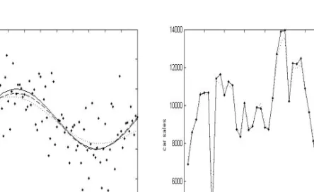
Artificial and real examples are provided to indicate the usefulness of the proposed method for the estimation of mean function in the presence of autocorrelation between data.

Keywords: Autoregressive process, cross validation function, hyper-parameters, kernel regression.

1. Introduction

A modified version of SVM (Vapnik, 1995, 1998) in a least squares sense has been proposed for classification in Suykens and Vanderwalle (1999). In LS-SVM concerning classification problems, we have regression interpretations and direct links to work in classical statistics.

In least squares support vector machine (LS-SVM) the solution is given by a linear system instead of a quadratic programming. The fact that LS-SVM has explicit primal-dual formu- lations has lots of advantages. For the application of LS-SVM the error terms are needed to be independently and identically distributed (error terms are iid).

Most nonparametric regression methods focus on estimating the mean function for various data types (Kim et al., 2008; Shim and Seok, 2008). The estimation of mean function from a data set is usually performed under the assumption that the error terms are iid (Juditsky et al., 1995). This assumption is not satisfied when the correlation is present in the given data (e.g. time series data), which leads to severe problems on the estimation of a model under the iid assumption.

† This research was supported by Korea SW Industry Promotion Agency (KIPA) under the program of Software Engineering Technologies Development and Experts Education.

1

Adjunct Professor, Department of Applied Statistics, Catholic University of Daegu, Kyungbuk 702-701, Korea.

2

Corresponding author: Professor, Department of Statistics, Dankook University, 126, Jukjeon-dong,

Suji-gu, Yongin-si, Gyeonggi-do 448-701, Korea. E-mail: [email protected]

In this paper, we consider the autoregressive model, where y _t −µ(x _t ) follows AR(p) process and x _t is the covariate vector including a constant 1. We propose a kernel method to take the autocorrelation into account and estimate the mean function under the AR model. The rest of this paper is organized as follows. The kernel method for autoregressive data is introduced in Section 2. In Section 3, the generalized cross validation function is given for the model selection. Also estimation method for AR(1) and AR(2) coefficient is presented. In Section 4 we perform the numerical studies through artificial and real examples. In Section 5 we give the conclusions.

2. Kernel method for autoregressive data

Let the given data set be denoted by {x _t , y _t } ⁿ _t=1 , with x _t ∈ R ^d including a constant 1 and y t ∈ R, we consider the autoregressive model,

Φ ^p (B)(y t − µ(x t )) = e t , t = 1, 2, · · · , n, (2.1) where Φ ^p (B) is a polynomial in back-shift operator B with parameters ρ _i , i = 1, · · · , p, such that Φ ^p (B)y _t = y _t − ρ ₁ y _t−1 − ρ ₂ y _t−2 − · · · − ρ _p y _t−p , and e _t is assumed to follow independently normal distribution (0, σ ² ). Throughout this paper we assume that y _t ’s are known to follow AR(p) process such that Φ ⁰ (B)(y 1 − µ(x 1 )) = e 1 , Φ ¹ (B)(y 2 − µ(x 2 )) = e 2 ,

· · · , Φ ^p−1 (B)(y p − µ(x p )) = e p , Φ ^p (B)(y t − µ(x t )) = e t , t = p + 1, p + 2, · · · , n. The mean function of y t given x t is given as E(y t |x t ) = µ(x t ).

The negative log likelihood of the given data can be expressed as (constant terms are omitted)

L(µ) =

p

X

t=1

(Φ ^t−1 (B)(y t − µ(x t ))) ² +

n

X

t=p+1

(Φ ^p (B)(y t − µ(x t ))) ² (2.2)

The mean function can be estimated by a linear model, µ(x) = ω ⁰ φ(x), conducted in a high dimensional feature space. Here the feature mapping function φ(·) : R ^d − > R ^d

^f

maps the input space to the higher dimensional feature space where the dimension d _f is defined in an implicit way. It is well known that φ(x _i ) ⁰ φ(x _j ) = K(x _i , x _j ), which are obtained from the application of Mercer’s conditions (1909). Then the estimates of ω is obtained by minimizing the regularized negative log likelihood,

L(ω) =

p

X

t=1

(Φ ^t−1 (B)(y t − ω ⁰ φ(x t ))) ² +

n

X

t=p+1

(Φ ^p (B)(y t − ω ⁰ φ(x t ))) ² + λ

2 ||ω|| ² (2.3) where λ is a nonnegative constant which controls the tradeoff between the goodness-of-fit on the data and ||ω|| ² . The representation theorem (Kimeldorf and Wahba, 1971) guarantees that the minimizer of the regularized negative log likelihood to be µ(x) = Kα for some vector α. For AR(1) the likelihood (2.3) is written as

L(α) =

n

X

t=2

(y _t − K(x t , x)α − ρ(y _t−1 − K(x t−1 , x)α) ² (2.4)

+(y ₁ − K(x ₁ , x)α) ² + λ

2 ||ω|| ² .

For AR(2) the likelihood (2.3) is written as

L(α) =

n

X

t=3

(y t − K(x t , x)α − ρ 1 (y t−1 − K(x t−1 , x)α − ρ 2 (y t−2 − K(x t−2 , x)α) ²

+ (y 1 − K(x 1 , x)α) ² + (y 2 − K(x 2 , x)α − ρ 1 (y 1 − K(x 1 , x)α) ² + λ

2 ||ω|| ² (2.5) Now the problem (2.3) becomes obtaining α to minimize

L(α) = (y ^∗ − K ^∗ α) ⁰ (y ^∗ − K ^∗ α) + λ

2 α ⁰ Kα, (2.6)

where

y ^∗ =









 y ₁ y 2 − ρy 1

.. . y n − ρy n−1









 , K ^∗ =











K ₁ K 2 − ρK 1

.. . K n − ρK n−1











f or AR(1),

y ^∗ =















y 1

y 2 − ρ 1 y 1

y 3 − ρ 1 y 2 − ρ 2 y 1

.. .

y n − ρ 1 y n−1 − ρ 2 y n−2













 , K ^∗ =















K 1

K 2 − ρ 1 K 1

K 3 − ρ 1 K 2 − ρ 2 K 1

.. .

K n − ρ 1 K n−1 − ρ 2 K n−2















f or AR(2),

and K _i is the i -th row of K such that K _i = K(x _i , x).

The estimates of α for the mean function can be found as

α = (K b ^∗ K ^∗ + λK) ⁻¹ K ^∗ y ^∗ , (2.7) which leads µ = K(K b ^∗ K ^∗ + λK) ⁻¹ K ^∗ y ^∗ = A µ y ^∗ .

y ^∗ can be written as y ^∗ = B ρ y with

B ρ =















1 0 0 · · · 0

−ρ 1 0 · · · · · · 0

0 −ρ 1 0 · · · 0

.. .

0 0 · · · · · · 0 − ρ 1















f or AR(1),















1 0 0 · · · 0

−ρ 1 1 0 · · · · · · 0

−ρ 2 −ρ 1 1 0 · · · 0

.. .

0 0 · · · · · · −ρ ₂ − ρ ₁ 1















f or AR(2).

Given x _t , the predicted value of µ(x _t ) is obtained as

µ(x b t ) = K(x t , x)(K ^∗ K ^∗ + λK) ⁻¹ K ^∗ B ρ y. (2.8)

3. AR coefficient estimation and model selection

In the mean function estimation, we should find the optimal values of hyper-parameters (λ and other tuning parameters included in the kernel K) and the estimate of ρ or (ρ 1 and ρ 2 ) for the estimation of µ = K b α. We denote a set of hyper-parameters by θ. b

Under the assumption that the estimate of ρ or (ρ 1 and ρ 2 ) is given, the optimal values of hyper-parameters can be chosen by minimizing the generalized cross validation function (Golub et al., 1979):

GCV (θ) = ny(I − A _µ B _ρ ) ² y

(n − tr(A µ B ρ )) ² . (3.1)

Under the assumption that the optimal values of hyper-parameters are given, the estimate of ρ for AR(1) is obtained by the conditional least squares method as follows,

ρ = b P n

t=2 (y t − b µ(x t ))(y t−1 − µ(x b t−1 )) P n

t=2 (y _t−1 − µ(x b _t−1 )) ² , (3.2) where µ(x b _t ) is the estimate of µ(x _t ) given the previous estimate of ρ and the optimal values of hyper-parameters obtained from GCV function (3.1).

For AR(2) the estimates of ρ ₁ and ρ ₂ can be obtained as respectively,

ρ b ₁ = r 1 − r 1 r 2

1 − r ₁ ² and ρ b ₂ = r 2 − r ₁ ²

1 − r ₁ ² , (3.3)

where r 1 =

P n

t=2 (y _t − µ(x b _t ))(y _t−1 − µ(x b _t−1 )) P n

t=1 (y t − µ(x b t )) ² and r 2 = P n

t=3 (y _t − µ(x b _t ))(y _t−2 − µ(x b _t−2 )) P n

t=1 (y t − b µ(x t )) ² . Thus the optimal values of hyper-parameters for the mean estimation and the estimate of ρ or (ρ ₁ and ρ ₂ ) are obtained iteratively as follows:

1. Set the initial value of ρ or (ρ ₁ and ρ ₂ ).

2. Obtain the optimal values of the hyper-parameters from GCV function (3.1).

3. Obtain the estimate of ρ or (ρ ₁ and ρ ₂ ) from (3.2) or (3.3).

4. Reiterate 2.-3. until convergence.

4. Numerical studies

We illustrate the performance of the mean estimation method based on the kernel method for autoregressive data through a simulated data set and a real data set.

Example 1. For the first example, we consider the autoregressive model, y 1 = µ(x 1 ) + e 1 , y 2 − µ(x 2 ) = ρ 1 (y 1 − µ(x 1 )) + e 2 ,

y t − µ(x t ) =ρ 1 (y t−1 − µ(x t−1 )) + ρ 2 (y t−2 − µ(x t−2 )) + e t , t = 3, · · · , 100

where ρ ₁ = 0.2, ρ ₂ = −0.7 x _t = t/100, µ(x _t ) = 1+sin(2πx _t ), e _t follows a normal distribution N (0, 0.5 ² ). The Gaussian kernel functions are utilized for the mean function estimation in this example. For the data set of Figure 4.1 (Left), λ and the kernel parameter are selected as 0.1 and 0.25, respectively, by GCV function (3.1) with the final estimates of (ρ 1 , ρ 2 ) = (0.1846, -0.7235). Figure 4.1 (Left) shows true mean functions (solid line) and estimated mean functions (dashed line) by proposed method, and estimated mean functions (dotted line) by LS-SVM which assumes iid errors, imposed on the scatter plots of 100 data points of y t ’s in a data set. In Figure 4.1 (Left) we can see that the proposed method seems to represent the behavior of mean function of given data better than LS-SVM. We repeated the above procedure 100 times (we generated 100 data sets) to have the root mean squared error (RMSE)s for the true mean functions as follows,

RMSE µ = v u u t

1 100

100

X

t=1

(µ t − µ b t ) ² .

For the proposed method we obtained the average of 100 RMSE _µ ’s and their standard error as 0.0859 and 0.0021, respectively. For LS-SVM we obtained the average of 100 RMSE _µ ’s and their standard error as 0.1163 and 0.0039, respectively. The smaller values of RMSE _µ s indicate that the proposed method works better than LS-SVM on the mean function estimation in this example.

Figure 4.1 Mean function estimation for Example 1 (Left) and Example 2 (Right)

Example 2. For the second example, we use the car sales data set of the brand name Sonata which is available at www.autotimes.co.kr. The data set consists of the number of Sonatas sold in each month from January 2006 to April 2009. We assumed AR(1) model for this data set.

y 1 = µ(x 1 ) + e 1 , y t − µ(x t ) = ρ(y t−1 − µ(x t−1 )) + e t , t = 2, · · · , 40

where y _t is the standardized car sales (Y _t ), x _t1 is the Sonata’s price at t -th month and x _t2 is KOSPI (Korea composite stock price index) at t -th month which is assumed to affect the car sales. The Gaussian kernel functions are utilized for the mean function estimation in this example. λ and the kernel parameter are selected as 0.001 and 0.25, respectively.

Figure 4.1 (Right) shows true mean functions (solid line) and estimated mean functions (dashed line) by proposed method, and estimated mean functions (dotted line) by LS-SVM which assumes iid errors, imposed on the scatter plots of 40 data points of Y t ’s in a data set.

The estimate of ρ is obtained as 0.1877, which implies that the previous car sales provides a small positive effect on the present car sales. We obtained the root mean squared error (RMSE) such as

RMSE µ = v u u t 1 40

40

X

t=1

(Y t − b Y t ) ² .

By the proposed method we obtained RMSE µ as 4.9432 and 226.0812 by LS-SVM. The smaller value of RMSE µ indicates that the proposed method works better than LS-SVM on the mean function estimation in this example.

5. Conclusions

In this paper, we dealt with estimating the mean functions for autoregressive model and obtained cross validation functions for the proposed method. Through the examples we showed that the proposed method yields the satisfying results. We also found that the proposed method has an advantage of an easy model selection method such as GCV func- tion. Also an advantage of easy extension to the heteroscedastic autoregressive model by incorporating a doubly penalizing method.

References

Golub, G. H., Heath, M. and Wahba, G. (1979). Generalized cross validation as a method for choosing a good ridge parameter. Technometrics, 21, 215-223.

Juditsky, A, Hjalmarsson, H., Benveniste, A., Deylon, B., Ljung, L., Sj¨ oberg, J. and Zhang, Q. (1995).

Nonlinear Black-box modelling in system identification: Mathematical foundations. Automatica, 31, 1725-1750.

Kim, M. S., Park, H. J., Hwang, C., and Shim, J. (2008). Claims reserving via Kernel machine. Journal of Korean Data & Information Science Society, 19, 1419-1417.

Kimeldorf, G. S. and Wahba, G. (1971). Some results on tchebycheffian spline functions. Journal of Math- ematical Analysis and its Applications, 33, 82-95.

Mercer, J. (1909). Functions of positive and negative type and their connection with theory of integral equations. Philosophical Transactions of Royal Society, A, 415-446.

Shim, J. and Seok, K. H. (2008). Kernel poisson regression for longitudinal data. Journal of Korean Data

& Information Science Society, 19, 1353-1360.

Suykens, J. A. K. and Vanderwalle, J. (1999). Least square support vector machine classifier. Neural Processing Letters, 9, 293-300.

Vapnik, V. N. (1995). The nature of statistical learning theory, Springer, New York.

Vapnik, V. N. (1998). Statistical learning theory, John Wiley, New York.