Stability Analysis of Concrete Shear Wall System with Opening

개구부를 갖는 전단벽의 안정해석

Stability Analysis of Concrete Shear Wall System with Opening

이 수 곤^* 김 순 철^** 송 창 영^*** 송 상 용^****

Lee, Soo-Gon Kim, Soon-Chul Song, Chang-Young Song, Sang-Yong

Abstract

A concrete shear wall system is commonly adopted in high-rise residential apartment buildings. In the construction stage, a rectangular opening is often made for the convenience of horizontal movement of workers, and construction materials and equipment. In the case of safety or stability assessment of a shear wall, the cutout part can be a critical factor. Finite element method is adopted to investigate the elastic stability behavior of the perforated unit shear wall. The key analysis parameters are the cutout location and its size. The effect of out-of-plane bending and horizontal shear are also examined in the stability analysis.

요 지

철근콘크리트조 고층아파트의 경우 흔히 전단벽식 구조시스템을 채택하게 된다. 이때에는 작업자의 이동과 재료나 장비의 수평 운반 편의상 세대간의 내력벽에 직 4각형 형태의 개구부를 설치할 때가 많 다. 이와 같은 개구부는 화재등의 재난시에 신속한 대피용 통로로 이용하도록 하는 경우도 있다. 전단 벽의 개구부는 구조체의 안전이나 안정을 위협하는 중요한 요소로 될 수 있으므로 설계시나 안전검토 에서 반드시 검토해야할 사항이다. 이번 연구는 개구부를 갖는 직 4각형 전단벽의 탄성안정에 관한 것 이다. 연구에서는 유한 요소법을 이용하였고 수치해석의 중요 변수는 개구부의 위치와 크기이다. 또한 연직 하중에 의한 균등 압축응력은 물론 휨 모멘트에 의한 응력 및 수평 전단력이 판의 임계응력에 미 치는 영향도 검토하였다. 끝으로 비재하면의 구속이 전단벽의 안정성에 미치는 영향도 검토하였다.

Keywords : Shear Wall, Rectangular Opening, Plane Stress Analysis, Elastic Critical Stress, Finite Element Method, Iteration Method

핵심 용어 : 전단벽, 직 4각형 개구부, 평면 응력해석, 탄성 임계응력, 유한요소법, 반복법

1)

* 전남대학교 건축학부 명예교수 ** 동신대학교 건축공학부 교수 *** (주)한국구조물안전원 대표이사

**** 비젼 구조연구소 연구원

2)

E-mail: [email protected], 011-607-6323

•본 논문에 대한 토의를 2005년 12월 31일까지 학회로 보내 주시면 2006년 4월호에 토론결과를 게재하겠습니다.

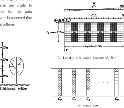
Fig. 1 Schematic view of example shear building

(a) Loading and cutout location (A, B,···)

(b) cutout size Fig. 2 Shear wall unit

1. Introduction

For the high-rise residential apartment build- ings, a concrete shear wall system is commonly adopted. During the construction stage of this shear wall system, a rectangular opening is usu- ally made in the wall (see Fig.1) for easy and rapid movement of construction workers, mate- rials and equipment. The cutout part is usually filled with cement bricks just before the final stage of room finishing. In this case, one can not expect perfect monolithic shear wall behav- ior especially when it is subjected to wind or earthquake induced horizontal load. This sug- gests that the perforated part in the shear wall can be a critical factor in the structural design or safety assesment of multi-story shear wall buildings.

Finite element method is adopted to inves- tigate the elastic stability behavior of The per- forated unit shear wall shown in Fig. 1. In the wall, cutout location and its size are made to change. The example shear wall has the ratio a/t = 270cm/18cm = 15 >10 and so it is assumed that unit shear wall satisfies Kirchhoff hypothesis.

2. Scope of the study

Fig. 2 shows the shear wall unit chosen for the stability analysis by finite element method.

In the same figure, two analysis parameters and their change patterns are also shown. As can be seen in the figure, α denotes the maximum flexural to the uniform gravity stress ratio, which is made to change from zero to 0.6 with subinterval 0.2 And β^, horizontal shear to gravity force ratio is to change from zero to 0.15 with subinterval 0.05. In the same figure, A, B, C and D designate the locations where the cutout is made. The symbols, C₀, C₁, ⋯, C₈ de- note the size of the perforated part. For example, C₀ means the wall without opening and C1 means the wall with an opening of 0.9m (horizontal) × 0.3m (vertical).

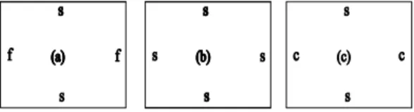
Fig. 3 shows the assumed boundary conditions

s : simple supported edge, f : free edge, c : clamped edge

Fig. 3 Boundary conditions

(a) Element under in-plane edge force

(b) Displacement component Fig. 4 Rectangular element for the shear wall unit. As can be seen in the

figure, the loaded edges are simply supported for all of the cases. One can easily expect that the behavior of the plate with the boundary conditions of Fig. 3(a) will be similar to that of a column with simply supported ends. In the shear wall buildings, the deformation of the unloaded edges can be restrained by the col- umns or by the walls which form right angles to the unloaded edges in the horizontal plan.

To take these facts into consideration, un- loaded edges are assumed to be either simply supported or completely fixed.

3. Displacement function and element stiffness matrices

3.1 Displacement function

Fig. 4(a) shows a thin rectangular element under the in-plane edge forces and Fig. 4(b) shows three displacement components at a typ- ical node " i ". For 12 degrees of freedom, the element displacement function, w is usually assumed to have the following form

w = A0+ A1x+ A2y + A3x²+ A4xy+ A5y²+ A6x³ + A7x²y+ A8xy²+ A9y³+ A10x³y+ A11xy³

(1)

The constants, A0, A₁, A₂, ⋯, A₁₁can be expressed in terms of nodal displacement components

and the result leads to

w = [ f1, f2, ⋯, f12]

{

}

( e = 1/8, ε = x/a, η = y/b)

f1= e(1- ε)( 1 -η)( 2 -ε²- η²- ε - η) f2= e(1- ε)( 1 -η)( 1 -ε²)a

f3= e(1- ε)( 1 -η)( 1 -η²)b

f4= e(1- ε)( 1 +η)( 2 -ε²- η²- ε - η)

Table 1 Flexural stiffness matrix, _{[k ]b}

D 60ab

60p +60p^{- 1}-42-12μ

b( 60p + 6 + 24μ) b²(80p+16-1 6μ) *p= (a/b)² symm.

a( 60p^{- 1}+6+24μ) 60μab a²(80p^{- 1}+16-16μ) 30p -60p^{- 1}-42+12μ b( 30p - 6 - 24μ) a( - 60p^{- 1}-6+ 6μ) k1, 1

k4, 2 b²(40p-16+1 6μ) 0 k2, 1 k2, 2

-k4, 3 -k5, 3 a²(40p^{- 1}-4+4μ) -k3, 3-k3, 2 k3, 3

30p -30p^{- 1}+42-12μ b( - 30p + 6 -6μ) a( - 30p^{- 1}+6-6μ) k10, 1 k10, 2 -k10, 3 k1, 1

-k_{7, 2} b( 20p + 4 - 4μ) 0 k_{11, 1} k_{11, 2} -k_{11, 3}-k_{2, 1} k_{2, 2}

-k7, 3 k8, 3 a^{2( 20p}+4-4μ) -k12, 1-k12, 2k12, 3 -k3, 1 k3, 2 k3, 3

-60p+ 30p^{- 1}-42+12μ b( - 60p - 6 +6μ) a( - 30p^{- 1}-6+24μ) k7, 1 k7, 2 -k7, 3 k4, 1 -k4, 2 -k4, 3 k1, 1

-k10, 2 b²(40p-4+4μ ) 0 k8, 1 k8, 2 -k8, 3 -k5, 1 k5, 2 k5, 3 -k2, 1 k2, 2

-k_{10, 3} -k_{11, 3} a²(40p^{- 1}-16+16μ) -k_{9, 1}-k_{9, 2} k_{9, 3} -k_{6, 1} k_{6, 2} k_{6, 3} k_{3, 3} -k_{3, 2} k_{3, 3}

f5= e(1- ε)( 1 +η)( 1 -ε²)a

f6=- e(1- ε)( 1 +η)( 1 -η ²)b (3) f7= e(1+ ε)( 1 +η)( 2 -ε²- η²+ ε + η) f8=- e(1+ ε)( 1 -η)( 1 -ε²)a

f9=- e(1+ ε)( 1 +η)( 1 -η²)b

f10= e(1+ ε)( 1 -η)( 2 -ε²- η²+ ε - η) f11=- e(1+ ε)( 1 -η)( 1 -ε²)a

f12= e(1+ ε)( 1 -η)( 1 -η²)b 3.2 Element stiffness matrices

The flexural strain energy stored in an ele- ment with sides 2a × 2b is given by

U = 1

2 ⌠

⌡

b - b

⌠⌡

a

- a{ φ}^T[ D]{ φ}dxdy (4) in which curvature vector, { φ } and elasticity matrix,

[ D ] are given by

{ φ} = ꀊ

ꀖ ꀈ

︳︳

︳︳

︳︳

︳

︳︳

︳︳

︳︳

︳

∂²w

∂x²

∂²w

∂y² 2 ∂²w

∂x∂y ꀋ

ꀗ ꀉ

︳︳

︳︳

︳︳

︳

︳︳

︳︳

︳︳

︳

(5.a)

[ D] = Et³ 12(1-υ²)

ꀎ ꀚ

︳︳

︳

ꀏ ꀛ

︳︳

︳

1 υ 0

υ 1 0

0 0 0.5( 1 -υ) (5.b)

in which ν denotes Poisson's ratio. The external work for the element is given by

W = 1

2{ δ }^T[k ]{ δ } + ⌠⌡

b - b

⌠⌡

a

- a{ α }^T[N ]{ α }dxdy (6)

in which rotation vector, { α } and in-plan force set, [ N ] are given by

{ φ} =

{

}

[

]

[

]

Equating the strain energy for the element to the external work and using Eq. (2) and (3), one obtains

[k] = [k ]b- q[k ]g (8)

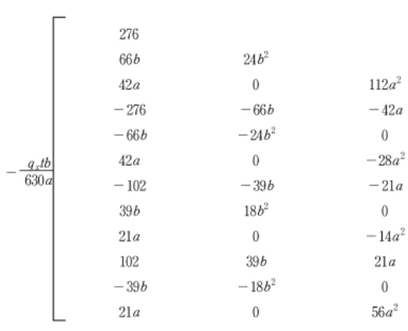
Table 2 Geometric stiffness matrix, _{[k ]g}

- qxtb 630a

276

66b 24b² symm.

42a 0 112a²

- 276 - 66b - 42a k_{1, 1}

- 66b -24b² 0 k2, 1 k2, 2

42a 0 -28a² -k3, 1 -k3, 2 k3, 3

- 102 - 39b - 21a k10, 1 k10, 2 -k10, 3 k1, 1

39b 18b² 0 k_{11, 1} k_{11, 2} -k_{11, 3}-k_{2, 1} k_{2, 2}

21a 0 -14a² -k12, 1 -k12, 2 k12, 3 -k3, 1 k3, 2 k3, 3

102 39b 21a k7, 1 k7, 2 -k7, 3 k4, 1 -k4, 2 -k4, 3 k1, 1

- 39b -18b² 0 k8, 1 k8, 2 -k8, 3 -k5, 1 k5, 2 k5, 3 -k2, 1 k2, 2

21a 0 56a² -k_{9, 1} -k_{9, 2} k_{9, 3} -k_{6, 1} k_{6, 2} k_{6, 3} k_{3, 3} -k_{3, 2} k_{3, 3}

Table 3 Critical load coefficients for the plate of Fig.3(a) _{qcr= k ⋅D/b}²_{, ( D = Et}³_/12(1-υ²), υ = 0.25)

α = 0.0, cutout location A

β = 0.0 β = 0.05 β = 0.10 β = 0.15

C0 8.84115 8.65017 8.17191 7.53615

⋮ ^{․ ․ ․ ․}

C6 6.90300 6.07464 5.16384 4.41522

C7 6.68529 5.79654 4.83741 4.07484

C8 6.41745 5.64246 4.67244 3.86703 α = 0.2, cutout location B

β = 0.0 β = 0.05 β = 0.10 β = 0.15

C0 8.35434 7.91613 7.37631 6.81705

⋮ ^{․ ․ ․ ․}

C6 6.68556 6.44202 5.99895 5.46912 C7 6.47451 6.30666 5.87799 5.32197

C8 6.25761 6.20460 5.79825 5.20920

in which flexural stiffness matrix, [k ]b and geo- metric stiffness matrix, q[k ]_g are given by follow- ing tables.

4. Elastic critical load

In the present study, the unit shear wall with sides 2.7m × 8.1m is subdivided into 9 × 27 square element as shown in Fig. 2. The plane stress analysis of plate under the loading condition together with opening and boundary conditions is performed to determine the in-plane force set, [ N ] (see Eq. 7.b), which enables one to obtain geometric stiffness ma- trix for each element.

The structure stiffness matrix for the plate is obtained by combining the element stiffness ma- trices consecutively. The application of boun- dary conditions to the assembled matrix leads to

( [ K]b- λ[ K]g){ △} = { 0} (9)

where △ denotes the nodal displacement vector for the whole plate. The least eigenvalue, or the critical load factor λcr can be determined by standard ei- genvalue iteration technique, for which above equation

is transformed into

( [ K]^{- 1}b [K] g- 1

λ[ I ]{ △} = { 0} (10)

where [ I ] is the identity matrix.

Some of the critical load coefficients, k de-

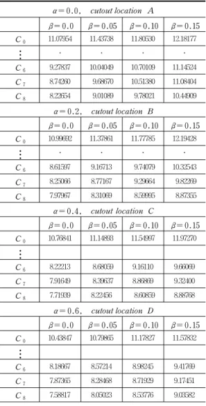
Table 4 Critical load coefficients for plate of Fig.3(b)

qcr= k ⋅D/b², ( D = Et³/12(1-υ²), υ = 0.25)

α = 0.0, cutout location A

β = 0.0 β = 0.05 β = 0.10 β = 0.15 C0 11.07954 11.43738 11.80530 12.18177

⋮ ^{․ ․ ․ ․}

C6 9.27837 10.04049 10.70109 11.14524 C7 8.74260 9.68670 10.51380 11.08404 C8 8.22654 9.01089 9.78021 10.44909

α = 0.2, cutout location B

β = 0.0 β = 0.05 β = 0.10 β = 0.15 C0 10.99692 11.37861 11.77785 12.19428

⋮ ^{․ ․ ․ ․}

C6 8.61597 9.16713 9.74079 10.32543 C7 8.25066 8.77167 9.29664 9.82269 C8 7.97967 8.31069 8.59995 8.87355

α = 0.4, cutout location C

β = 0.0 β = 0.05 β = 0.10 β = 0.15 C0 10.76841 11.14893 11.54997 11.97270

⋮

C6 8.22213 8.68059 9.16110 9.66069 C7 7.91649 8.39637 8.86869 9.32400 C8 7.71939 8.22456 8.60859 8.88768

α = 0.6, cutout location D

β = 0.0 β = 0.05 β = 0.10 β = 0.15 C0 10.43847 10.79865 11.17827 11.57832

⋮

C6 8.18667 8.57214 8.98245 9.41769

C7 7.87365 8.28468 8.71929 9.17451

C8 7.58817 8.05023 8.53776 9.03582

Table 5 Critical load coefficients for plate of Fig.3(c) _{qcr= k ⋅D/b}²_{, ( D = Et}³_/12(1-υ²), υ = 0.25)

α = 0.0, cutout location A

β = 0.0 β = 0.05 β = 0.10 β = 0.15 C0 11.88261 12.27609 12.69612 13.12686

⋮ ^{․ ․ ․ ․}

C6 9.83421 10.70865 11.52081 12.20292 C7 9.10656 10.15497 11.12841 11.89116 C8 8.39349 9.21969 10.05831 10.82493

α = 0.2, cutout location B

β = 0.0 β = 0.05 β = 0.10 β = 0.15 C0 11.81358 12.24486 12.69477 13.16223

⋮ ^{․ ․ ․ ․}

C6 9.22329 9.78732 10.37619 10.97946

C7 8.72388 9.20655 9.70857 10.22634

C8 8.26515 8.52327 8.78157 9.04329

α = 0.4, cutout location C

β = 0.0 β = 0.05 β = 0.10 β = 0.15 C0 11.65680 12.09618 12.55833 13.04379

⋮ ^{․ ․ ․ ․}

C6 8.86302 9.33633 9.82296 10.31967

C7 8.51769 8.96850 9.39897 9.80946

C8 8.31042 8.67987 8.94924 9.16164

α = 0.6, cutout location D

β = 0.0 β = 0.05 β = 0.10 β = 0.15 C0 11.41776 11.85048 12.30795 12.79098

⋮ ^{․ ․ ․ ․}

C6 8.75700 9.19035 9.64953 10.13310

C7 8.39259 8.84961 9.32859 9.82251

C8 8.07768 8.59158 9.12402 9.64692

termined by repeating above procedures, are listed in Table 3 through 5.

5. Discussion of the results

To date no literature is available to compare the results of the present study except in the cases of plates with C₀ and α = β = 0.0 (No per-

foration, no horizontal shear and uniform com- pression).

When the unloaded edges are free, the be- havior of the plate with C0 and α = β = 0.0 should be similar to that of a column with simply supported ends. In this case, the critical load intensity per unit length of the plate will be given by

q_cr= k π²D

a² , ( k = 1.0)

(a) Loading

(b) Critical load coefficient Fig. 5 Fig. 2(a) plate with _C0

From Table 3, one can confirm that the critical load coefficient for the case C0 and α = β = 0.0 is k = 8.8411/9 = 0.9823, which yields the lower bound error, -1.8%. The loading condition for the plate without opening can be represented by Fig. 5 (a). The changes in critical load co- efficient are visualized in Fig. 5 (b). It is no- ticed that the wall (or the column) becomes more unstable as the magnitude of lateral shear force, Q increases.

When the plate edges are simply supported, the stability analysis is somewhat easy. In this case critical load coefficient, k is given

( a = 2.7m, b = 8.1m, m = 1)

k = ( mb a + a

mb)²= 100

9 = 11.111

The finite element analysis(Table 4) shows critical load coefficient, k = 11.079, which is 0.28%

less than the exact value.

According to Cox's study, the critical load co- efficient, k for the plate shown in Fig. 3(a)

k = 4 3[ 4( a

b ) + 3 4 ( b

a )²+ 2] = 12.25 9

The finite element analysis(Table 5) is given by k = 11.8826 resulting in the lower bound error of 3.07%. From the above comparisons of 3 types of plate, one can easily guess the possibility of design aid role of the present study.

Examinations of Table 3 through 5 reveal that critical load coefficient change is decreas- ing function of cutout size, which can be said the expected results. Also the tables suggest that the cutout part around the unloaded edges is to be avoided when possible. One thing note worthy, in Table 4 and 5, is the increase of horizontal shear force, Q (increase of β ) makes the plate more stable, which may be explained with the diagonal tensile force induced by Q.

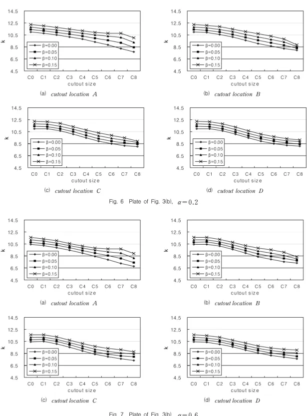
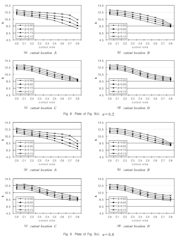
For easy understanding of plate stability, the changes in the critical load coefficient of Table 4 and 5, that is the coefficients for the boun- dary conditions of Fig. 3(b) and (c), are vi- sualized in Fig. 6, Fig. 7, Fig. 8 and Fig. 9.

(a) cutout location A 4.5

6.5 8.5 10.5 12.5 14.5

C0 C1 C2 C3 C4 C5 C6 C7 C8

cutout s iz e

k β=0.00

β=0.05 β=0.10 β=0.15

(b) cutout location B 4.5

6.5 8.5 10.5 12.5 14.5

C0 C1 C2 C3 C4 C5 C6 C7 C8

cutout s iz e

k β=0.00

β=0.05 β=0.10 β=0.15

(c) cutout location C 4.5

6.5 8.5 10.5 12.5 14.5

C0 C1 C2 C3 C4 C5 C6 C7 C8

cutout s iz e

k β=0.00

β=0.05 β=0.10 β=0.15

(d) cutout location D 4.5

6.5 8.5 10.5 12.5 14.5

C0 C1 C2 C3 C4 C5 C6 C7 C8

cutout s iz e

k β=0.00

β=0.05 β=0.10 β=0.15

Fig. 6 Plate of Fig. 3(b), α = 0.2

(a) cutout location A 4.5

6.5 8.5 10.5 12.5 14.5

C0 C1 C2 C3 C4 C5 C6 C7 C8

cutout s iz e

k β=0.00

β=0.05 β=0.10 β=0.15

(b) cutout location B 4.5

6.5 8.5 10.5 12.5 14.5

C0 C1 C2 C3 C4 C5 C6 C7 C8

cutout s iz e

k β=0.00

β=0.05 β=0.10 β=0.15

(c) cutout location C 4.5

6.5 8.5 10.5 12.5 14.5

C0 C1 C2 C3 C4 C5 C6 C7 C8

cutout s iz e

k β=0.00

β=0.05 β=0.10 β=0.15

(d) cutout location D 4.5

6.5 8.5 10.5 12.5 14.5

C0 C1 C2 C3 C4 C5 C6 C7 C8

cutout s iz e

k β=0.00

β=0.05 β=0.10 β=0.15

Fig. 7 Plate of Fig. 3(b), α = 0.6

(a) cutout location A 4.5

6.5 8.5 10.5 12.5 14.5

C 0 C1 C2 C3 C4 C5 C6 C7 C8

c u to u t s iz e

k β=0.00

β=0.05 β=0.10 β=0.15

(b) cutout location B 4.5

6.5 8.5 10.5 12.5 14.5

C 0 C1 C2 C3 C4 C5 C6 C7 C8

c u to u t s iz e

k β=0.00

β=0.05 β=0.10 β=0.15

(c) cutout location C 4.5

6.5 8.5 10.5 12.5 14.5

C 0 C1 C2 C3 C4 C5 C6 C7 C8

c u to u t s iz e

k β=0.00

β=0.05 β=0.10 β=0.15

(d) cutout location D 4.5

6.5 8.5 10.5 12.5 14.5

C 0 C1 C2 C3 C4 C5 C6 C7 C8

c u to u t s iz e

k β=0.00

β=0.05 β=0.10 β=0.15

Fig. 8 Plate of Fig. 3(c), α = 0.2

(a) cutout location A 4.5

6.5 8.5 10.5 12.5 14.5

C 0 C1 C2 C3 C4 C5 C6 C7 C8

c u to u t s iz e

k β=0.00

β=0.05 β=0.10 β=0.15

(b) cutout location B 4.5

6.5 8.5 10.5 12.5 14.5

C 0 C1 C2 C3 C4 C5 C6 C7 C8

c u to u t s iz e

k β=0.00

β=0.05 β=0.10 β=0.15

(c) cutout location C 4.5

6.5 8.5 10.5 12.5 14.5

C 0 C1 C2 C3 C4 C5 C6 C7 C8

c u to u t s iz e

k β=0.00

β=0.05 β=0.10 β=0.15

(d) cutout location D 4.5

6.5 8.5 10.5 12.5 14.5

C 0 C1 C2 C3 C4 C5 C6 C7 C8

c u to u t s iz e

k β=0.00

β=0.05 β=0.10 β=0.15

Fig. 9 Plate of Fig. 3(c), α = 0.6

참고문헌

1. S.G. Lee, S.C. Kim and J.G. Song, "Critical Loads of Square Plate under Different Inplane Load Configurations on Opposite Edges", Journal of Structural Stability and Dynamics, 1(2), 283-291, 2000.

2. N. Yamaki ; Buckling of a Rectangular Plates under Locally Distributed Forces Applied on the Two Opposite Edges, Handbook of Structural Stability, CRC of Japan, 1981.

3. H.L. Lox, The Buckling of Thin Plate in Compress- ion, Handbook of Structural Stability, CRC of Japan, 1981.

4. M.L. Sharp, "Behavior of Plates under Partial Edge Loading", "Proceedings of the sessions re-

lated to Steel Structures, Structures Congress '89", San Francisco, 215-224, 1989.

5. M.Z. Khan and K.C. John, "Buckling of Plates un- der Partial Edge Loadings", J. Struct. Eng, Mech.

Div. Proc ASCE EM 5, 67-86, 1962.

6. N. White and W.S. Cottingham, "Stability of Plates under Partial Edge Loadings", J. Struct. Eng, Mech. Div. Proc ASCE EM 5, 67-86, 1962.

7. A. Chajes, "Principle of Structural Stability Theory", Prentice-Hall, Inc., Englewood Cliffs, NJ, 1987.

8. J.S. Kinney, "Indeterminate Structural Analysis", Assison Wesley Publishing Co., Massachusetts, USA, 1975.

(접수일자：2005년 6월 2일)