The impact of public rental housing projects on neighborhood housing markets in Korea
A spatio-temporal approach
1
Kim, Chun-Il*
Abstract
After the Korean government initiated the provision of the permanent public rental housing in 1989, there has been a variety of policy measures to provide decent housing for low-income households. As of 2009, the ratio of the public rental housing to the total housing became 4.8 percent. It is widely agreed that the nation needs to build more public housing and to target a wider range of the types of households. However, the expansion of such development projects has resulted in worries and oppositions in the impacted neighborhoods, which have insisted that such developments bring about negative impacts on the adjacent neighborhoods. This study explores the impact of recently developed public rental housing (“ Kukmin” rental housing) on the nearby housing markets. The paper adopts a quasi-experimental design to deal with the possible endogeneity for the construction of public rental housing by adopting an extended treatment to the canonical difference-in-difference method. This research finds that the public housing projects increase the value of surrounding properties.
Keywords : Public rental housing, NIMBY, Difference-in-differences, AITS
Ⅰ. Introduction
There is a variety of policy tools for the provision of decent housing for low-income households all over the countries. In the Unites States, starting from the late 1960s, the federal government has provided approximately 300,000 homes for low-income households
* 주택도시금융공사 주택도시금융연구원 금융정책팀 연구위원 ([email protected])
on a yearly basis. Public rental housing also plays an important role in housing welfare in Korea by providing the minimum level of housing service at a low cost. In 1989, starting with the construction of permanent rental housing, the Korean government continued to supply public rental housing to improve the level of low-income housing welfare. However, the expansion of such development projects has resulted in worries and oppositions in the impacted communities, which insist that the projects cause negative impacts from the socio-economic perspectives (Carter et al., 1998; Hirsch, 2009).
Unlike other commodities, houses exert external impacts on the surrounding area because they are fixed in location. Negative views on the public rental housing have been a major risk factor for the rental housing policy. The residents of the apartment complex proved to be reluctant to build public rental housing in the neighboring area (Hong and Lee, 2006). The “Not In My Back Yard (NIMBY)” phenomenon has long been a major threat to housing planners and policy practitioners who want to push forward initiating subsidized housing development at the community and regional scale.
Ashey and Kean (1999) reported that the contributing factors to this NIMBY Syndrome as concerns on property value depreciation, abrupt changes in community characteristics, increases in local public service needs, increases in fiscal expenditures, and deterioration of community homogeneity. Social misbehavior conducted by some particular income or racial/ethnic groups might be one of the major concerns and fears (Ellen et al., 2012;
McNulty and Holloway, 2000; Roncek et al., 2000).
Do the subsidized housing developments have negative (or positive) impacts on the neighborhood’s housing prices? Empirical studies show mixed results. As for the U.S.
cases, early papers by Lee et al. (1999) and Cummings and Landis (1993) discovered negative impacts while others found positive impacts on the community’s home prices.
LIHTC projects crowd out the near-by new rental housing construction, and the effect
leads to the increase in the adjacent unsubsidized housing prices at the aggregate census
tract level. Those opposite results could simply be due to the different context of the
study areas. However, the main reason should be the difference in the research
methodologies depending on the target area, type of public rental housing, and spatial
range of spillover effects. In the Korean context, Moon et al. (2006) showed that there
is a negative perception of public rental housing in the city of Busan, but it does not
cause a fall in the surrounding land price. Hong and Lee (2006) concluded that the
prices of apartment units in the private market within a 500-meter radius of Kukmin
rental housing projects do not fall due to the construction of the public rental housing.
Moon and Lee (2008) revisited the same research topic as in the 2006 study using a difference-in-difference method, showing that public rental housing decreases the surrounding land prices. Kim and Choi (2009) utilized multilevel models to confirm that there is no statistical significance in the effect of rental housing complex (separated type and mixed type) on house price. Park and Kwon (2009) concluded that Kukmin rental housing had a negative effect on the newly-built private housing complex within the 600-meter range. The study by Kim (2013) found that the better the location of the rental housing complex, the more positive effect it has on the prices of the surrounding apartments.
This study discusses the methodological limitations of previous researches and suggests research methodologies that are often found in overseas literature but not yet applied in domestic research.
Ⅱ. AITS-DID Methodology and Its Extension
Typical hedonic models have limitations on drawing causal interpretations. Specifically, the ex ante market condition is not fully considered in the empirical specification, which may result in the selection bias. In other words, the cross-section hedonic models fail to fully address the direction of the causality. The selection of the construction sites is endogenous. If the units are constructed in neighborhoods where the values of residential properties keep decreasing, the impacts can be more negative. Similarly, if the projects are placed in locations that are improving, the impacts can be upward-biased.
Galster et al. (1999) proposed the adjusted interrupted time series/difference-in-difference (AITS-DID) to investigate the causal relationship between the provision of subsidized housing development and the local housing market in order to overcome the weakness of the hedonic price method
1. As they investigated the impact of the Section 8 Housing Choice Voucher projects on the adjacent housing prices in Baltimore County, Maryland, they introduced the concept of “micro-neighborhood”, which is assumed to be affected by large housing projects and can be thought of as the residents’ spatial boundary of daily life. They showed that (1) in the 500-feet radius micro-neighborhoods with high-income
1 AITS stands for Adjusted Interrupted Time Series.
whites the Section 8 housing exerts positive impacts on the vicinity of the projects, and (2) the impacts are negative in the low-income micro-neighborhoods.
The AITS-DID approach is a deviation from the canonical hedonic method in order to investigate the casual relationship of the subsidized housing program on the existing housing market at the very local level. The model considers the neighborhoods’ price levels and trends before and after the subsidized housing units are provided. It sets up the housing price as the dependent variable, and housing characteristics as the independent variables, which follows the similar specification to the traditional hedonic regression.
When the regression suffers from the multicollinearity problem due to the inclusion of a large number of independent variables, the model can use the spatial fixed effects to control for the location and amenity variation. For example, the census tract dummy variables are entered in the right hand side of the equation.
The big difference between the traditional difference-in-difference approach and the AITS-DID modeling is that the latter incorporates both the pre-post and the impact-control design. For example, the study by Castells (2010), which used the simple DID method to estimate the impacts of HOPE VI redevelopment projects on their immediate vicinity, included dummy variables that indicate whether or not properties were sold within certain distances from such developments. Then, the paper interpreted the coefficients of the dummy variables as the treatment effects. Galster et al. (2004) argued that the simple DID methods are flawed because they do not control for the trajectory of housing prices.
Suppose the growth rate of the housing prices around the subsidized housing projects is higher, relative to the non-impact area, and the LIHTC developers choose those locations with higher expected capital gains. Then, even if a relative increase in the post-impact price levels may be due to LIHTC, the effects of the post-intervention on the adjacent housing prices might contain both the general upward price trend around the LIHTC locations and the positive spillover effect from the LIHTC projects.
In the AITS-DID framework, housing sales are divided into the two categories: the
impact sales and the control sales. The impact sales are the ones the locations of which
are within the radius of the subsidized housing projects. On the other hand, the control
sales are beyond the micro-neighborhood boundary. This stage implies the impact-control
design. As for the pre-post set-up, the impact sales are again divided into the two
groups: the sales before the completion of the subsidized housing projects and the ones
after the completion of such projects. As a result, the model has two types of dummy
variables. These two explain the difference in the price levels before and after the
impact. The pre-price level variable takes on the value of 1 if the sales occurred before the impact. Similarly, the post-price level variable takes on the value of 1 if the sales made after the impact. Notice that those two dummy variables are only for the impact sales. All the other control sales take on the value of 0 for the two variables. As for the trend variables, we can introduce the other two variables. The pre-trend variable is a continuous variable that takes on the time duration between the sales date and the completion of the affordable housing projects of interest. The same logic applies to the post-trend variable.
Private housing units sold are designated as the “impact” sales if they are within the 250-meter radius from the project. The buffer distance reflects the concept of “micro- neighborhood”, which is operationally defined as the very local level of spatial boundary (Galster, 1999). This research is to test whether or not a public housing development has a spillover effect within the micro-neighborhood in which direction. The housing sales beyond this concentric ring buffer (from 250-meter to 500-meter region) are the controls for this quasi-experiment research.
One challenge to the unbiasedness of the causal effect of the housing development on the adjacent housing units is the possible endogeneity due to any other factors correlated with the placement of the low-income housing projects. As for the U.S. LIHTC cases, the LIHTC developers presumably choose neighborhoods where the long-term housing price appreciation is anticipated (Di, 2013). In addition, the LIHTC developers might locate their developments in qualified census tracts (QCTs) with greater tax credit allocation (Baum-Snow, 2009). This situation is similar to the Korean context. The government could not fully ignore the location of the projects. The government needs to designate the project locations that are both cheaper and not very far from urban areas in order to draw potential tenants. This paper address the endogeneity issue by including the “pre-impact time trend” variable. This variable takes on the values of 1, 2, 3, etc (in years) from the beginning of the study period, that is 1987. Houses that were not affected (beyond the 150-meter radius) take on the value of 0. Moreover, the “post-impact time trend” variable is added to address the ex post housing price movement after the completion of the LIHTC projects. This variable takes on the value of 1, 2, 3, etc (in years) from the subsidized year of the nearby LIHTC project. Finally, the hedonic equation for the housing price is formed as follows:
ln (1)
where ln is the logged sales price of private housing units. indicates the pre-impact and the post-impact dummy variables ( indexes the pre and the post of the public housing development within the public housing micro-neighborhood boundary).
includes the pre-time trend and the post-time trend variable for the impact housing sales.
is a set of the structural characteristics of housing unit. Finally, captures unobservable neighborhood amenities ( indexes the administrative districts (“dong” in Korean) in the study area). With being [ ]’, the treatment effect is simply
× in the precentage point term.
The difference of the canonical AITS-DID from the method that is employed in this study is as follows:
ln (2)
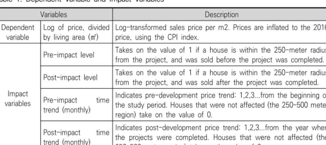
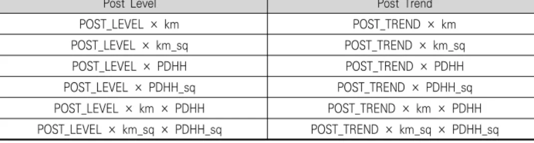
where is the interaction terms of (1) post-impact level variable, the distance to the project( , and the number of housing units in the project ( ); and (2) post-impact time trend variable, the distance to the project(, and the number of housing units in the project( ). Now, the treatment effect is not just a scalar, but a function of (1) the number of housing units in the public housing project and (2) the distance to the project. To estimate the model as in equation (2), the dependent variable and the impact variables are formulated as in Table 1 and Table 2.
Variables Description
Dependent
variable Log of price, divided
by living area (㎡) Log-transformed sales price per m2. Prices are inflated to the 2016 price, using the CPI index.
Impact variables
Pre-impact level Takes on the value of 1 if a house is within the 250-meter radius from the project, and was sold before the project was completed.
Post-impact level Takes on the value of 1 if a house is within the 250-meter radius from the project, and was sold after the project was completed.
Pre-impact time trend (monthly)
Indicates pre-development price trend: 1,2,3...from the beginning of the study period. Houses that were not affected (the 250~500 meter region) take on the value of 0.
Post-impact time trend (monthly)
Indicates post-development price trend: 1,2,3...from the year when the projects were completed. Houses that were not affected (the 250~500 meter region) take on the value of 0.
Table 1. Dependent Variable and Impact Variables
Post Level Post Trend
POST_LEVEL × km POST_TREND × km
POST_LEVEL × km_sq POST_TREND × km_sq
POST_LEVEL × PDHH POST_TREND × PDHH
POST_LEVEL × PDHH_sq POST_TREND × PDHH_sq
POST_LEVEL × km × PDHH POST_TREND × km × PDHH POST_LEVEL × km_sq × PDHH_sq POST_TREND × km_sq × PDHH_sq Table 2. Interaction Terms
Ⅲ. Descriptive Statistics
The 48 public housing projects are selected for the study. The average number of the units in the project is 251 with the minimum of 101 and the maximum of 550 (Table 3). The average number of floors of the projects is 14.42. The typical triple-deckers housing in New England region in the United States are three- to four-story buildings.
Public rental housing buildings in Korea are typically high-rise properties. The average building age is 7 years.
Variable N Mean Std. Dev. Min Max
# units in the project 48 251.15 117.79 101 550
# of floors 48 14.42 2.33 8 21
Building age (in years) 48 7.02 2.20 3 10
Table 3. Public housing projects
Only private high-rise apartment units are considered for the private housing markets.
There are other types of housing in Korea, such as single-detached, three- or four-story buildings, and so forth. Approximately 50 percent of the total housing stock is apartment units, and the frequency of sales for the other types is relatively thin. The “NIMBYism”
is typically occur around the apartment complexes in the form of residents’ collective opposition.
The average unit apartment price, measured by the sale prices divided by the living area, is approximately 5,846 thousand Won per square meter, which is about 5,500 USD.
The living area is about 80 square meters. The number of the floor is around seven on
average. The building age is 14.7 years. There are 918 units in the apartment complex
on average. The number of the housing units in the complex is the proxy for the size of the complex, which is one of the important factors to determine the apartment prices in Korea. Typically, consumers prefer large-size complexes because larger one contains non-residential uses more, and occupants value the accessibility to those functions. The distance to the nearest subway station from the apartment complex is 831 meters on average.
In the impact area sample (in the 250-radius areas from the public housing projects), the unit sale price is slightly less, which is 5,623 thousand Won. The living area is about 81 square meters. The number of the floor is around seven on average. The building age is 11 years. There are 658 units in the apartment complex on average. The distance to the nearest subway station from the apartment complex is 934 meters on average.
Variable N Mean Std. Dev. Min Max
Unit Price(Korean Won) 10,339 5,623,454 1,521,407 1,243,578 16,100,000
Area(m²) 10,339 81.07 118.53 7.26 8496.00
# of floor 10,339 7.53 4.20 -1.00 24.00
Building age(year) 8,834 11.14 4.71 4.00 29.00
# of units in APT complex 8,834 658.43 367.01 6.00 1466.00
Distance to subway station(m) 10,339 934.94 667.73 174.71 2906.88 Table 4. Housing sales data: impact area
On the other hand, in the control area sample (in the 250- to 500-meter region), the unit sale price is 6,007 thousand Won. The living area is about 78.5 square meters, which is slightly smaller than the one in the impact area. The number of the floor is around 6.8 on average. The building age is 16.9 years. There are 1,080 units in the apartment complex on average. The distance to the nearest subway station from the apartment complex is 758 meters on average. In sum, the private housing units near the public housing location is smaller and older in comparison with the units in the control area.
In addition, the apartment complexes in the outside area contain more housing units, as
opposed to the complexes in the area adjacent to the public housing projects.
Variable N Mean Std. Dev. Min Max Unit Price(Korean Won) 14,319 6,006,862 2,746,532 1,535,272 19,400,000
Area(m²) 14,319 78.50 22.84 12.38 188.13
# of floor 14,319 6.83 4.38 1.00 25.00
Building age(year) 14,103 16.94 9.98 2.00 37.00
# of units in APT complex 14,103 1080.86 836.38 6.00 2678.00 Distance to subway station(m) 14,319 757.63 586.62 17.89 4401.27 Table 5. Housing sales data: control area
Ⅳ. Regression Results and Impact Estimates
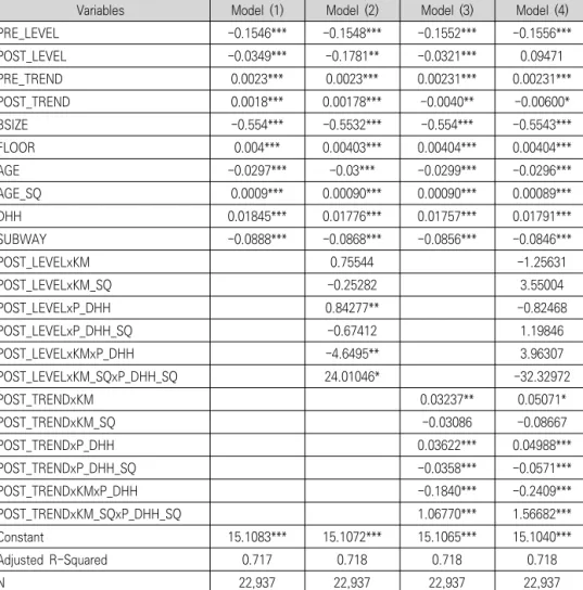
Nine models were originally considered to find the best model for the equation (2) above (Table 6 and Table 7). Model (1) pre and post impact level and trend variables and other important covariates. Before the construction of public housing projects, nearby housing prices were increasing. This effect is stable throughout the other models.
The living area is negatively associated with the unit price. Building age is negatively related to the unit price, but the squared term of the age is positive and highly statistically significant. In Korea, as apartment building ages to the particular point in time, the prices tend to go up again. This tendency reflects the expected possibility to redevelop the properties, and the newly-developed units tend to sell more.
Model (2) includes some interaction terms that comprise the post level variable, the
distance to the project, and the project size. Similarly, Model (3) includes some interaction
terms that comprise the post trend variable, the distance to the project, and the project
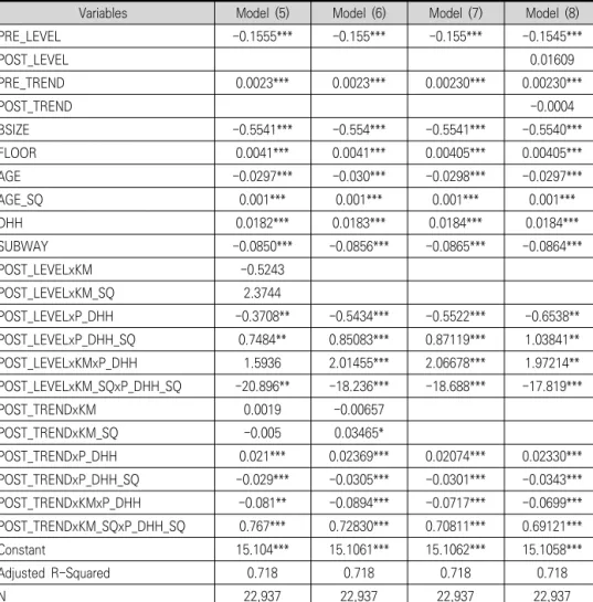
size. Model (4) contains both of the variable sets. In Model (5), the post level and the
post trend variables are removed because there are a great deal of multicollinearity with
the interaction terms. From Model (5), the interaction terms of the post level variable
and the distance variables are removed to end up with Model (6). The final model to
calculate the treatment effects is Model (7) because the post-level and the post trend
variables are not significant in Model (8).
Variables Model (1) Model (2) Model (3) Model (4)
PRE_LEVEL -0.1546*** -0.1548*** -0.1552*** -0.1556***
POST_LEVEL -0.0349*** -0.1781** -0.0321*** 0.09471
PRE_TREND 0.0023*** 0.0023*** 0.00231*** 0.00231***
POST_TREND 0.0018*** 0.00178*** -0.0040** -0.00600*
BSIZE -0.554*** -0.5532*** -0.554*** -0.5543***
FLOOR 0.004*** 0.00403*** 0.00404*** 0.00404***
AGE -0.0297*** -0.03*** -0.0299*** -0.0296***
AGE_SQ 0.0009*** 0.00090*** 0.00090*** 0.00089***
DHH 0.01845*** 0.01776*** 0.01757*** 0.01791***
SUBWAY -0.0888*** -0.0868*** -0.0856*** -0.0846***
POST_LEVELxKM 0.75544 -1.25631
POST_LEVELxKM_SQ -0.25282 3.55004
POST_LEVELxP_DHH 0.84277** -0.82468
POST_LEVELxP_DHH_SQ -0.67412 1.19846
POST_LEVELxKMxP_DHH -4.6495** 3.96307
POST_LEVELxKM_SQxP_DHH_SQ 24.01046* -32.32972
POST_TRENDxKM 0.03237** 0.05071*
POST_TRENDxKM_SQ -0.03086 -0.08667
POST_TRENDxP_DHH 0.03622*** 0.04988***
POST_TRENDxP_DHH_SQ -0.0358*** -0.0571***
POST_TRENDxKMxP_DHH -0.1840*** -0.2409***
POST_TRENDxKM_SQxP_DHH_SQ 1.06770*** 1.56682***
Constant 15.1083*** 15.1072*** 15.1065*** 15.1040***
Adjusted R-Squared 0.717 0.718 0.718 0.718
N 22,937 22,937 22,937 22,937
Table 6. Regression Results: Model (1)~(4)
※ * p<0.1, ** p<0.05, *** p<0.01
Variables Model (5) Model (6) Model (7) Model (8)
PRE_LEVEL -0.1555*** -0.155*** -0.155*** -0.1545***
POST_LEVEL 0.01609
PRE_TREND 0.0023*** 0.0023*** 0.00230*** 0.00230***
POST_TREND -0.0004
BSIZE -0.5541*** -0.554*** -0.5541*** -0.5540***
FLOOR 0.0041*** 0.0041*** 0.00405*** 0.00405***
AGE -0.0297*** -0.030*** -0.0298*** -0.0297***
AGE_SQ 0.001*** 0.001*** 0.001*** 0.001***
DHH 0.0182*** 0.0183*** 0.0184*** 0.0184***
SUBWAY -0.0850*** -0.0856*** -0.0865*** -0.0864***
POST_LEVELxKM -0.5243
POST_LEVELxKM_SQ 2.3744
POST_LEVELxP_DHH -0.3708** -0.5434*** -0.5522*** -0.6538**
POST_LEVELxP_DHH_SQ 0.7484** 0.85083*** 0.87119*** 1.03841**
POST_LEVELxKMxP_DHH 1.5936 2.01455*** 2.06678*** 1.97214**
POST_LEVELxKM_SQxP_DHH_SQ -20.896** -18.236*** -18.688*** -17.819***
POST_TRENDxKM 0.0019 -0.00657
POST_TRENDxKM_SQ -0.005 0.03465*
POST_TRENDxP_DHH 0.021*** 0.02369*** 0.02074*** 0.02330***
POST_TRENDxP_DHH_SQ -0.029*** -0.0305*** -0.0301*** -0.0343***
POST_TRENDxKMxP_DHH -0.081** -0.0894*** -0.0717*** -0.0699***
POST_TRENDxKM_SQxP_DHH_SQ 0.767*** 0.72830*** 0.70811*** 0.69121***
Constant 15.104*** 15.1061*** 15.1062*** 15.1058***
Adjusted R-Squared 0.718 0.718 0.718 0.718
N 22,937 22,937 22,937 22,937
Table 7. Regression Results: Model (5)~(8)
※ * p<0.1, ** p<0.05, *** p<0.01
Table 8 shows different treatment effect numbers as the distance and the number of
units in the project vary. For example, the price gap between the impact and the control
area gets smaller by 10.55 pp for the private apartment 40 meters away from the 100-unit
project. At the same location, the treatment effect is positive and increasing up to the
point where the number of units in the project is around 260. Then, the effect picks up
again as the number of project units increases. The price gap between the impact and
the control areas is reduced by approximately 8 percent points to 13 percent points,
which implies that the public housing development actually exert some positive spillovers
to the adjacent housing markets.
Figure 1. Treatment Effects by the Selected Levels of the Number of Housing Units in the Projects Treatment
effects (pp) Distance to the project (km)
0.04 0.06 0.1 0.16 0.2 0.22
# housing units in the project
(in thousands)
0.10 10.55 10.91 11.60 12.52 13.07 13.33
0.12 10.00 10.43 11.22 12.26 12.85 13.1
0.14 9.52 10.01 10.89 12.02 12.64 12.91
0.16 9.11 9.65 10.62 11.82 12.44 12.70
0.18 8.76 9.35 10.41 11.65 12.25 12.48
0.20 8.48 9.12 10.24 11.51 12.07 12.27
0.22 8.26 8.95 10.13 11.40 11.90 12.05
0.24 8.11 8.84 10.07 11.32 11.74 11.83
0.26 8.02 8.79 10.06 11.27 11.59 11.61
0.28 7.99 8.80 10.11 11.25 11.45 11.38
0.30 8.02 8.87 10.21 11.27 11.32 11.16
0.32 8.12 9.01 10.36 11.31 11.20 10.93
0.34 8.28 9.20 10.56 11.38 11.09 10.70
Table 8. Treatment effects by the housing project size and the distance to the project
Figure 1 illustrates this non-linear relationship in detail. When the housing units in
the project is 200, the treatment effect is increasing in the range from 40 meters to 240
meters. But, as the housing units in the project increase to 340 units, the treatment effect
is maximized around the distance of 150 meters. Then, the effect decrease again. This non-linear relationship clearly shows that the effect is the interplay between the negative perception and the positive amenity improvement generated from the public housing development. As the number of units in the project becomes larger, the positive benefit turns to be concave down with respect to the distance to the project. As the number of units in the project becomes larger, the treatment effect becomes smaller.
But the speed of the price appreciation after the construction of the project gets bigger(Figure 2). At the very edge of the impact area, around 17 months after the construction, the price gap between the impact and the control area is expected to disappear regardless of the number of housing units in the project.
Figure 2. Impact Estimates (Distance to the project = 240 meters)