Comparison of Improved Explicit Method and Predictor Correct α-Method

전체 글

(1)한국복합신소재구조학회 논문집 제3권, 제4호, 2012년 12월 J. Korean Soc. Adv. Comp. Struc. Vol. 3, No. 4, pp. 1-9, December 2012 DOI http://dx.doi.org/10.11004/kosacs.2012.3.4.001. ISSN 2093-5145. 개선된 명시적 방법과 예측수정 α-Method방법의 비교 권민호1 · 정우영2 경상대학교 토목공학과 교수1, 강릉원주대학교 토목공학과 교수2. Comparison of Improved Explicit Method and Predictor Correct α-Method 1. 2. Kwon, Min-Ho · Jung, Woo-Young 1. Professor, Department of Civil Engineering, ERI, Gyeongsang National University, Jinju, South Korea Professor, Department of Civil Engineering, Gangneung-Wonju National University, Gangneung, South Korea. 2. A bstract: Dynamic application lower mode response is of interest, however the higher modes of spatially discretized equations generally do not represent the real behavior. Some implicit algorithms, therefore, are introduced to filter out the high-frequency modes. The objective of this study is to introduce the P-method and PC α-method to compare that with dissipation method and Newmark method through the stability analysis and numerical example. PC α-method gives more accuracy than other methods because it based on the α-method inherits the superior properties of the implicit α -method. In finite element analysis, the PC α-method is more useful than other methods because it is the explicit scheme and it achieve the second order accuracy and numerical damping simultaneously. Key Words: Dynamic, α-Method, P-Method, PC α-Method, Newmark method. 1. Introduction In many dynamic application only lower mode response is of interest. The higher modes of spatially discretized equations generally do not represent the real behavior. In addition, the presence of numerical errors will lead to the spurious growth of high mode response. Some implicit algorithms, therefore, are introduced to filter out the high-frequency modes such as the Wilson method, Houbolt's method, and the dissipation method. However, the Wilson method and Houbolt's methods damp out the lower frequency modes too strongly. The dissipation method developed by H. M. Hilber, et. al(1976) gives the desired numerical damping effect and second order accuracy. Even though dissipation method is unconditionally stable and second order, the implementation is more complicated than that of explicit method. Although the general Newmark method gives numerical damping, it has first order numerical damping, i.e., lower modes are too much damped out. To archive second order accuracy and numerical damping simultaneously, I. Miranda, R.M. Ferencz and T.J.R. Hughes(1989) developed the predictor-corrector -method(PC-method) based on the implicit dissipation method and S.Y. Chang(1997) also developed the P-method which is based on Newmark explicit method. The objective of this study is to introduce the P-method and PC α-method to compare that with. 주요어: α-Method, P-Method, PC α-Method, Newmark method Corresponding author: Jung, Woo-Young Department of Civil Engineering, Gangneung-Wonju National University, 7 Jukhun-gil, Gangneung, South Korea. Tel: +82-033-640-2421, Fax: +82-033-646-1391 , E-mail:[email protected] 투고일: 2012년 9월 12일 / 수정일: 2012년 10월 19일 / 게재확정일: 2012년 11월 29일. Korean Society for Advanced Composite Structures. 1.

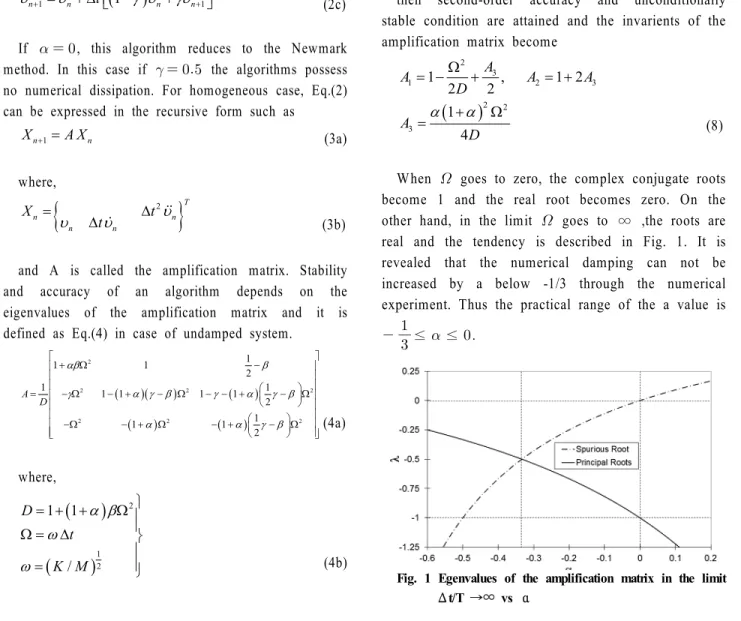
(2) Kwon, Min-hoㆍJung, Woo-Young. dissipation method and Newmark method through the stability analysis and numerical example.. 2. α-Method. where M is the mass matrix, K is the stiffness matrix, F is the vector of external force, is the displacement vector. Approximate solution of Eq.(1) is obtained as following M υ&&n +1 + (1 + α )Cυ&n +1 − α Cυ&n + (1 + α ) Kυn +1 − α Kυn = Fn +1+α ⎞ ⎠. (2a) (2b). υ&n +1 = υ&n + Δt ⎣⎡(1 − γ )υ&&n + γυ&&n +1 ⎦⎤. (2c). ⎦. If   , this algorithm reduces to the Newmark method. In this case if    the algorithms possess no numerical dissipation. For homogeneous case, Eq.(2) can be expressed in the recursive form such as X n +1 = A X n. (3a). where, Xn =. {υ. n. Δt υ&n. and A is called and accuracy of eigenvalues of the defined as Eq.(4) in. Δt 2 υ&&n. }. T. (3b). the amplification matrix. Stability an algorithm depends on the amplification matrix and it is case of undamped system.. ⎡ ⎤ 1 2 −β 1 ⎢1 + αβΩ ⎥ 2 ⎢ ⎥ ⎥ 1⎢ 1 ⎛ ⎞ 1 − (1 + α )( γ − β ) Ω 2 1 − γ − (1 + α ) ⎜ γ − β ⎟ Ω 2 ⎥ A = ⎢ −γΩ 2 D⎢ ⎝2 ⎠ ⎥ ⎢ ⎥ ⎛1 ⎞ ⎢ −Ω 2 − (1 + α ) Ω 2 − (1 + α ) ⎜ γ − β ⎟ Ω 2 ⎥ ⎝2 ⎠ ⎣⎢ ⎦⎥. general,. (5).   ≠ , therefore, the amplification. matrix has three non-zero eigenvalues. A consequence of convergence is that if  is in between 0 and   , then the characteristic equation has two complex conjugate roots   , principal roots, and a so-called. spurious ..     . root.  ,. Under. these. which. satisfy. circumstance. the. principal roots become. λ1,2 = A ± iB. (6). if  and  are taken as. β=. ⎤. υn +1 = υn + Δt υn + Δt 2 ⎢⎜ − β ⎟υ&&n + βυ&&n +1 ⎥ 2 ⎣⎝. det ( A − λ I ) = λ 3 − 2 A1λ + A2 λ − A3 = 0 In. The equation of motion for a linear system can be expressed as M υ&& + Cυ& + Kυ = F (1). ⎡⎛ 1. The characteristic equation of A is. 1 1 2 (1 − α ) γ = − α 4 2. (7). then second-order accuracy and unconditionally stable condition are attained and the invarients of the amplification matrix become. A1 = 1 −. Ω 2 A3 + , 2D 2. α (1 + α ) Ω 2. A2 = 1 + 2 A3. 2. A3 =. 4D. (8). When  goes to zero, the complex conjugate roots become 1 and the real root becomes zero. On the other hand, in the limit  goes to ∞ ,the roots are real and the tendency is described in Fig. 1. It is revealed that the numerical damping can not be increased by a below -1/3 through the numerical experiment. Thus the practical range of the a value is    ≤  ≤ . . (4a). where, ⎫ D = 1 + (1 + α ) βΩ 2 ⎪ ⎪ Ω = ω Δt ⎬ ⎪ 1 ⎪⎭ ω = ( K / M )2. 2. J. Korean Soc. Adv. Comp. Struc. (4b). Fig. 1 Egenvalues of the amplification matrix in the limit Δt/T →∞ vs α.

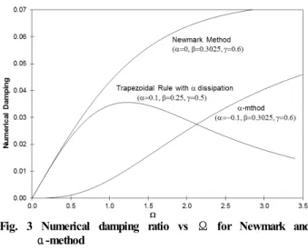
(3) Comparison of Improved Explicit Method and Predictor Correct α-Method. To compute numerical damping and numerical natural frequency, one can assume the response of the system as. υn = C1λ1n + C2 λ2n = C1e n ( A+ iB ) + C 2e n ( A−iB ) = e nA [G1 cos(nB) + G2 sin(nB )]. (9). The analytical solution for free vibration response is expressed as. υ ( nΔt ) = e −ξω nΔt ⎡⎣Gˆ1 cos (ωD Δt ) + Gˆ 2 sin(ωD Δt ) ⎤⎦ (10) If the viscous damping of system is ignored, the numerical damping and frequency can be derived as Eq.(11) through comparison Eq.(9) with Eq.(10).. ξ =−. ln( A2 + B 2 ) , 2ωΔt. ω=. 1 ⎛B⎞ tan −1 ⎜ ⎟ Δt ⎝ A⎠. (11). Spectral radius is an important measure of stability and dissipation. Fig. 2 illustrates the spectra vs Δt/T for the Trapezoidal rule, Newmark method, and α -method. Trapezoidal rule is unconditionally stable, but it doesn't have the numerical dissipation. The results of trapezoidal with α-dissipation and Newmark method have some numerical dissipation, however, it is not an effective damping mechanism. Only α -method has the desirable numerical dissipation. It becomes obviously in Fig. 3. Newmark method has not second-order damping, i.e., lower frequencies are damped out too strongly. It also shows that higher frequencies are not damped out effectively and lower frequencies are damped strongly in trapezoidal rule with α-dissipation.. Fig. 3 Numerical damping ratio vs Ω for Newmark and α-method. 3. Predictor-Corrector α-Method (PC α-Method) Predictor-Corrector algorithm naturally arises from Eq.(2). Predictor phase : 1 (1 − 2β ) Δt 2υ&&n 2 = υ&n + (1 − γ ) Δtυ&&n. υ%n +1 = υn + Δtυ&n + υ&%n +1. (12). Not likely α-method, time discrete equation of motion is taken at the predictor phase instead of    except acceleration term. Time discrete equation of motion : M υ&& + (1 + α ) Cυ&% − α Cυ& n +1. n +1. n. + (1 + α ) Kυ%n +1 − α Kυn = Fn +1+α. (13). Corrector phase :. υn +1 = υ%n +1 + βΔt 2υ&&n +1 υ&n +1 = υ&%n +1 + γΔtυ&&n +1. (14). For homogeneous case, Eq.(12)(14) can be changed in recursive form such as Eq.(3a). The amplification matrix of PC α-method is derived as ⎡ ⎤ ⎢ 1 ⎪⎧ ⎛ ⎛1 ⎞ ⎞ ⎪⎫⎥ 2 2 − β ⎨1 + ⎜ (1 + α ) (1 − γ ) 2ξΩ + (1 + α ) ⎜ − β ⎟ Ω2 ⎟ ⎬⎥ ⎢1 − βΩ 1 − β {2ξΩ + (1 + α ) Ω } 2 ⎪⎩ ⎝ ⎝2 ⎠ ⎠ ⎭⎪⎥ ⎢ ⎢ ⎥ ⎢ −γΩ 2 1 − γ {2ξΩ + (1 + α ) Ω 2 } 1 − γ ⎧⎪⎨1 + ⎜⎛ (1 + α ) (1 − γ ) 2ξΩ + (1 + α ) ⎛ 1 − β ⎞ Ω2 ⎟⎞ ⎪⎫⎬ ⎥ ⎜ ⎟ ⎢ ⎪⎩ ⎝ ⎝2 ⎠ ⎠ ⎭⎪ ⎥ ⎢ ⎥ ⎢ ⎥ ⎛1 ⎞ 2 − {2ξΩ + (1 + α ) Ω2 } − (1 + α ) (1 − γ ) 2ξΩ − (1 + α ) ⎜ − β ⎟ Ω2 ⎢ −Ω ⎥ ⎝2 ⎠ ⎣ ⎦. Fig. 2 Spectral Radius for Newmark and α-method. (15). The characteristic equation of the amplification matrix A becomes. det ( A − λ I ) = λ 3 − 2 A1λ + A2 λ − A3 = 0. (16). Vol. 3, No. 4, 2012. 3.

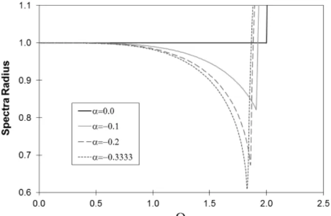
(4) Kwon, Min-hoㆍJung, Woo-Young. 4. P-Method where, ⎛ ⎞⎤ 1⎡ 1⎞ ⎛ A1 = 1 − ⎢ 2ξΩ (1 + α (1 − γ ) ) + Ω 2 ⎜ (1 + α ) ⎜ γ + ⎟ − βα ⎟ ⎥ 2⎣ 2⎠ ⎝ ⎝ ⎠⎦ ⎡ 1 ⎛ ⎞⎤ A2 = 1 − ⎢ 2ξΩ (1 + 2α (1 − γ ) ) + Ω 2 ⎜ γ − + 2α ( γ − β ) ⎟ ⎥ 2 ⎝ ⎠⎦ ⎣ ⎡ 1 ⎞⎤ ⎛ A3 = − ⎢ 2ξΩα (1 − γ ) + Ω 2α ⎜ γ − β − ⎟ ⎥ 2 ⎠⎦ ⎝ ⎣. (17). From Eq.(16)(17), stability analysis can be carried If  and  is defined as Eq.(7), the PC α-method becomes one parameter method and it has    second-order accuracy in the range of ∈    .    If  does not satisfy the Eq.(7), the algorithm becomes first-order accurate. Fig. 4 shows the stability limit of predictor -corrector method. And Fig. 5 indicate this method has the desired numerical damping effect, that is, second order damping mechanism.. If α is equal to zero in Eq.(2a), the α method becomes Newmark method. In the case of β equal to 0, the algorithm is energy conserving if   , whereas numerical dissipation presents if   . It is necessary to assume    to develop P-method since it is supposed to be explicit. To make α-function dissipation method,  is set to be 0.5 and the amplification matrix becomes ⎡ 1 ⎢ 1 ⎢ 1 2 1 ⎢ − Ω 1 − (1 + α ) Ω 2 2 2 ⎢ ⎢ 2 − (1 + α ) Ω 2 ⎢ −Ω ⎣. ⎤ ⎥ ⎥ 1 1 2 − (1 + α ) Ω ⎥ 2 4 ⎥ ⎥ 1 2 − (1 + α ) Ω ⎥ 2 ⎦ 1. (18). The characteristic equation and eigenvalues of the amplification matrix can be expressed as Eq.(19).. λ ( λ 2 − A1λ + A2 ) = 0. (19a). where, A1 = 2 − (1 + α ) Ω 2 ,. A2 = 1 − αΩ 2 , A3 = 0. λ1,2 = A ± iB. (19b). where, A = 1−. Fig. 4 Spectral Radius of the amplification matrix for PC α-method. 1 (1 + α ) Ω 2 , 2. B = Ω 1−. 1 2 (1 + α ) Ω2 (19c) 4. The algorithm is stable if and only if max≤  and the roots of the amplification matrix should be complex conjugate to make the solution realistic (sinusoidal response). Therefore, α value is bounded as 0≤α ≤. 2 −1 Ω. (20). In general, numerical damping and frequency are function of  and increasing function with increasing positive slopes for an integration method having frequency-proportional damping. Thus,  and   can be expressed as Fig. 5 Numerical damping for PC α-method. ξ = F (Ω), Ω = G (Ω). (21). By substituting Eq.(21) into Eq.(11) and A, B are 4. J. Korean Soc. Adv. Comp. Struc.

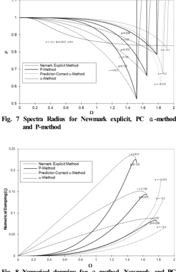
(5) Comparison of Improved Explicit Method and Predictor Correct α-Method. defined in Eq.(19b), one can obtain ⎛ 1 ⎞ ⎧⎪. ⎡ 2Ω F (Ω) ⎤ ⎫⎪. α = ⎜ 2 ⎟ ⎨1 − exp ⎢ − ⎥⎬ ⎝ Ω ⎠ ⎩⎪ ⎣ 1 − G (Ω) ⎦ ⎭⎪. (22). For simplicity,   and    are assumed to be an increasing polynomial function of  . F (Ω ) = pΩ q , G (Ω ) = r Ω s. (23). where p, q, r, and s are positive constants. In addition, q and s must be greater than 1 to become increasing function with increasing positive slope. The effects of p, q, r and s are investigated through parametric studies and is shown in Fig. 6. Comparing Fig. 6(a) and 6(b) with Fig. (6c) and 6(d), one can conclude that the variations of the constants p and q have larger effect on numerical damping than those of r and s. Fig. 6(a) indicates that the curve moves upward with the increase of p value and all the curves can archive the desired numerical damping. Fig. 6(b) shows that the algorithm has a desired numerical dissipation when q is greater than 3. Since the amount of the numerical damping is not affected by the coefficient of    , it is convenient to assume    as zero and the q is set to 3. Thus Eq.(22) is reduced to. α=. {. }. 1 1 − exp ⎡⎣ −2 p Ω 4 ⎤⎦ Ω2. The spectra radii and the numerical damping ratio of the P-method have been plotted in Fig. 7 and 8 Explicit Newmark method has a linear numerical damping which damp out low frequency too. The results of P-method indicate it has the desired numerical damping. The damping curve with almost coincides with the curve of the PC α-method  with    in less than 1.4 which has maximum  numerical dissipation. Therefore, P-method has the larger numerical damping effect than that of PC α -method.. Fig. 7 Spectra Radius for Newmark explicit, PC α-method and P-method. (24). Using Taylor's expansion, one can obtain a simple polynomial function of Eq.(24) such as ∞. α = ∑ ( −1). n +1. n =1. ∞. = ∑ ( −1) n =1. ⎡ ( 2 p )n ⎤ 4 n − 2 ⎢ ⎥Ω ⎣⎢ n ! ⎦⎥. n +1. ⎡k ⎤ pn ⎢ Δt 2 ⎥ ⎣m ⎦. 2 n −1. (25a) Fig. 8 Numerical damping for ρ-method, Newmark, and PC α-method. where, pn =. (2 p). n. n!. (25b). If only the first term of Eq.(25) is taken, it becomes. α = p1. k 2 Δt m. (26). 5. Comparison of Algorithms The spectra radius, numerical damping, and period error for the presented algorithms are compared in this section. The trapezoidal method, Newmark method, and α-method when parameters are set to Eq.(7) achieve the unconditionally stable, and Vol. 3, No. 4, 2012. 5.

(6) Kwon, Min-hoㆍJung, Woo-Young. 0.25. 0.25. 0.2. p=0.01 p=0.03 p=0.05 p=0.07 p=0.09. Numerical Damping. Numerical Damping Ratio. 0.2. 0.15. 0.1. r=0.01 r=0.03 r=0.05 r=0.07 r=0.09. 0.15. 0.1. 0.05. 0.05. 0. 0 0. 0.2. 0.4. 0.6. 0.8. 1. Ω. 1.2. 1.4. 1.6. 1.8. 0. 2. 0.2. (a) q=3, r=0.05 and s=3. 0.6. 0.8. 1. Ω. 1.2. 1.4. 1.6. 1.8. 2. 1.4. 1.6. 1.8. 2. (b) p=0.05, q=3 and s=3. 0.25. 0.25. 0.2. 0.2. q=1 q=2 q=3 q=4 q=5. 0.15. s=1 s=2 s=3. Numerical Damping. Numerical Damping. 0.4. 0.1. 0.05. s=4 s=5. 0.15. 0.1. 0.05. 0. 0 0. 0.2. 0.4. 0.6. 0.8. 1. 1.2. 1.4. 1.6. 1.8. 2. 0. 0.2. 0.4. 0.6. 0.8. (c) p=0.05, r=0.05 and s=3. 1. 1.2. Ω. Ω. (d) p=0.05, q=3 and r=0.05. Fig. 6 Parametric effects on variation of numerical damping vs. Ω. Newmark explicit, P-method, and PC α-Method are conditionally stable as Fig. 9. The PC α-method shows lager stability limit than those of Newmark Explicit method and P-method, however, P-method indicates larger numerical dissipation ability. Fig. 10 shows that Newmark explicit method, Newmark implicit method and 6 J. Korean Soc. Adv. Comp. Struc. Trapezoidal Rule damp out the lower frequency too much, on the other hand, α-method, PC α-method and P-method have a second order numerical damping mechanism and it also shows that the effect of numerical damping in α-method are not effective than that of PC α-method and P-method. It seems that α -method needs large time step to eliminate the high.

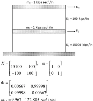
(7) Comparison of Improved Explicit Method and Predictor Correct α-Method. frequency term. From Fig. 11 one can observe that PC α-method are more accurate than the other method in the range of  ≤  ≤ . The numerical error of the P-method is closer to that of Newmark explicit method by increasing of  . It is obvious because P-method is derived from Newmark explicit method. The α-method have the second order numerical error before    and it is changed to the first order function. However, the numerical error of the P-method and PC α-method also is the second order function as they have the second order accuracy and numerical dissipation. That is, the numerical error of the P-method and the PC α-method rapidly grow up by the increasing of discretized time step. However, period error of α-method does not grow up rapidly because the error function becomes linear after   .. Fig. 11 Comparison of the Period Error. 6. Numerical Example A two story linear elastic shear building is considered. The unusual structure is intentionally chosen to have a high natural frequency in order to demonstrate the characteristic of the numerical dissipation. Fig. 12 shows the mode shapes and frequencies of the structure. It is subjected to initial displacement and the response becomes free vibration.. Fig. 9 Comparison of the Spectra Radius. K=⎡ ⎤, m= ⎡ ⎤ ⎢15100 −100 ⎥ ⎢1 0 ⎥ ⎢ −100 100 ⎥ ⎢0 1 ⎥ ⎣ ⎦ ⎣ ⎦ Φ=⎡ ⎤ ⎢ 0.00667 0.99998 ⎥ ⎢ 0.99998 −0.00667 ⎥ ⎣ ⎦. ω1,2 = 9.967, 122.885 rad / sec Fig. 12 The Examples Structure and Properties. Fig. 10 Comparison of the Numerical Damping. The initial condition for given structure is selected as the first mode shape add to 100 times of the second mode such as     . The exact solution for second floor displacement is in. Vol. 3, No. 4, 2012. 7.

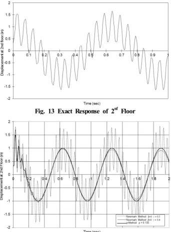
(8) Kwon, Min-hoㆍJung, Woo-Young. Fig. 13 and the numerical solutions are in Fig. 14, 15 and 16. The time step used in all the lgorithms is 0.01 sec. Fig. 15 demonstrates that P-method and PC α-method can effectively damp out the second mode. After about 0.2 sec, P-method eliminate the second mode completely. PC α-method damp out the second mode after about 0.5 sec. The Newmark(     ) method takes 0.2 and 0.4 sec to damp out the second mode. When    is used in Newmark method, the numerical dissipation is not appeared as discussed before. On the other hand, the α-method takes 1.4 sec to eliminate the second mode. Even though Newmark method damp out the second mode very quickly, the first mode also damped out strongly as Fig. 16 Obviously, the P-method can filter out the second mode very quickly and hardly affects the first mode at all. Actually, this result can be completely explained by the Fig. 8 since the  values for each mode are about 0.01 and 1.22 which correspond to about zero and 12% numerical damping. Thus the first mode is almost not affected and the second mode can be damped out very quickly.. Fig. 15 Numerical Solution by PC α-method and α-method. Fig. 16 Numerical Solution by Newmark Explicit and P-method. 7. Conclusions. Fig. 13 Exact Response of 2nf Floor. Fig. 14 Numerical Solution by Newmark(ϒ=0.5) and P-method. 8 J. Korean Soc. Adv. Comp. Struc. P-method and PC α-method, conditionally stable, have been introduced and are shown to possess significantly improved numerical damping. In particular, those methods are of second-order-accuracy and they are possible to achieve zero damping. It was shown that P-method and PC α-method possess better accuracy than the Newmark explicit method since all the introduced algorithms are second-order methods while the Newmark explicit method is first-order method. PC α-method gives more accuracy than other methods because it based on the α-method inherits the superior properties of the implicit α-method. Even though P-method has the second order accuracy and numerical damping, it is not efficient to be implemented in nonlinear MDOF system. Because the parameter α is expressed in terms of p 1, time.

(9) Comparison of Improved Explicit Method and Predictor Correct α-Method. step, and natural frequencies which are always changing during the time history analysis. i.e., the parameter α is not a constant and have to compute at the each time step. However, P-method can be applied to solve linear elastic MDOF system using modal superposition method. In spite of this limitation, it is still useful for pseudo-dynamic test methods since the spurious growth of higher mode response can be eliminated quickly by the numerical damping while lower modes are obtained accurately. In finite element analysis, the PC α-method is more useful than other methods because it is the explicit scheme and it achieve the second order accuracy and numerical damping simultaneously.. Acknowledgements This work was supported by the Natural Disaster Prevention Research Institute of Kangnung-Wonju National University, South Korea.. References Bathe K. J. and Wilson E. L. (1976) Numerical Meth.in Finite Element Analysis. Printice-Hall. Chang, S. Y. (1997) “Improved Numerical Dissipation for Explicit Methods in Pseudo-dynamic Test.” Earthquake Eng. and Struct. Dynamics, 26(9), pp.917-930. Hilber, H. M., Hughes T. J. R. and Taylor, R. L. (1977). “Improved Numerical dissipation for time integration algorithms in Structural Dynamics.” Earthquake Eng. and Struct. Dynamics, 5(3), pp.283-292. Miranda, I., Ferencz R. M. and Hughes, T. J. R. “An Improved Implicit-Explicit time Integration method for Structural Dynamics.” Earthquake Eng. and Struct. Dynamics, 18(5), pp.643-653.. Vol. 3, No. 4, 2012. 9.

(10)