Application of Artificial Neural Network method for deformation analysis of shallow NATM tunnel due to excavation

(1)

Application of Artificial Neural Network method for deformation analysis of shallow

NATM tunnel due to excavation

Jae-Ho LEE1*・ Shnichi AKUTAGAWA²・ Hong-Duk MOON³・ Heui-Soo

HAN4・ Ji-Hyeung YOO⁵・ Kwang-Yeun Kim⁵

1Dept. of Civil Engineering, Kyungpook National University(〒702- 701,Korea,Daegu,Puk-gu,Sankyuk-dong 1370) 2Dept. of Architecture and Civil Engineering, Kobe University(〒657-

0031,kobe,Nada-ku,Rokkoudai-cho 1-1) 3Dept. of Civil Engineering, Jinju National University(〒660-

758,Korea,Jinju,Chil-am-dong 150) 4Dept. of Civil Engineering, Kumoh Nat'l Institute of Tech.(〒730-

701,Korea,Gumi,Yangho-dong 1) 5Dept. of Civil Engineering, Kyungil University(〒712-

701,Korea,Gyeongsan,Hayang-eup,Buho-ri 33)

*E-mail: [email protected] Abstract: Currently an increasing number of urban tunnels with small overburden are excavated according to the principle of the New Austrian Tunneling Method (NATM). For rational management of tunnels from planning to construction and maintenance stages, prediction, control and monitoring of displacements of and around the tunnel have to be performed with high accuracy. Computational method tools, such as finite element method, have been and are indispensable tool for tunnel engineers for many years. It is, however, a commonly acknowledged fact that determination of input parameters, especially material properties exhibiting nonlinear stress-strain relationship, is not an easy task even for an experienced engineer. Use and application of the acquired tunnel information is important for prediction accuracy and improvement of tunnel behavior on construction. Artificial Neural Network (ANN) model is a form of artificial intelligence that attempts to mimic behavior of human brain and nervous system.

The main objective of this paper is to perform the deformation analysis in NATM tunnel by means of numerical simulation and artificial neural network (ANN) with field database. Developed ANN model can achieve a high level of prediction accuracy.

Key Words : NATM tunnel, Artificial neural network, Numerical simulation, Field database, Deformation analysis

1. Introduction

Successful planning, excavation, lining installation and maintenance of NATM tunnel demands prediction, control and monitoring of tunnel behavior, face stability, surface settlement, gradient and ground displacement with high accuracy.

Of several possible methods of incorporating tunnel construction information for this prediction accuracy and improvement of tunnel behavior, this paper proposes the Artificial Neural Networks

(Rumelhart et al., 1986, 1995). As this method requires firstly preparation of database that contains information to relate input parameters to output parameters, a database is created by performing the acquirement of field data. ANN model are then created studying the database and establishing selected relationships between input and output parameters.

This paper discussed the deformation analysis of NATM tunnel due to excavation stage using ANN analysis with the acquired FEM database and field data.

한국암반공학회 국제학술회의

2008 / 2008.10.21 - 10.23

(2)

2. Fundamental approach by ANN method

Data interpretation

•Parameter identification

•Predictive analysis

Construction and Monitoring Design

Database ANN model

Field investigation

Data interpretation

•Parameter identification

•Predictive analysis

Construction and Monitoring Design

Database ANN model

Field investigation

(a) Tunnel design and construction

Input Output

Data division Field database

Data processing

Tunnel behavior Tunnel

geometrics Ground condition Excavation / support system

Input Output

Data division Field database

Data processing

Tunnel behavior Tunnel

geometrics Ground condition Excavation / support system

(b) Process of ANN approach

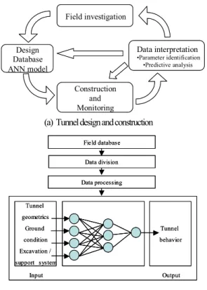
Fig. 1. ANN approach based tunnel designand construction

Survey and preliminary investigation.

Design tunnel structure.

Build a database using FEM.

Learn the database and make ANN models.

Construction and field measurement.

Data interpretation.

Identify key parameters from measurements using the built

ANN models.

Perform predictive analyses to ensure safety in all remaining stages.

Is it safe ?

Finished ? Yes No

No

Stop Start

Design modification. Proceed to next excavation stage.

Fig.2 Flowchart of an observational method using ANN.

technique. Procedures related to ANN are depicted by Gothic font.

Numerical analysis or empirical method carried out for the validity the selected support system with preliminary ground estimation on design stage. However, it is difficult to understand that ground estimation over all tunnel section before construction. For reason them, it is carried out the investigation of tunnel information with various measures, as the geology and geo-mechanical properties of the rocks, tunnel face observation recorded, the presence of underground water, surface settlement, subsurface displacement and the tunnel displacement. It is important the using and application of the acquired tunnel information for this prediction accuracy and improvement of tunnel behavior on construction. ANN model is well suited the problem of classification and understanding of the acquired data. Fig. 1 shows a scheme of ANN model for prediction of tunnel behavior. The neural network in the input layer receives tunnel geometric, ground condition, excavation method and support system, as input values. Tunnel behaviors are to be determined from output values.

In case of numerical analusis, use of ANN approach can be regarded as one form of back analyses conducted in the framework of a modern observational method, which is depicted in Fig.2. An act of parameter identification as measurement data become available in field should be performed as quickly as possible for safety management reasons in the data interpretation section in the diagram.

In order to make this possible, one has to build a database beforehand and let ANN learn about the database in order to establish a trustful ANN model that relates input parameters rationally to output parameters. This learning process, which is the most time consuming, can be performed before construction starts in a design stage, as depicted in Fig.2.

3. Outline of artificial neural network model

ANN is a form of artificial intelligence that attempts to mimic the behavior of the human brain and nervous system. Back Propagation Neural Network (BPNN) is the most popularly used ANN and it is well suited for problem of classification, prediction, adaptation control, system identification, and so on (Rumelhart et al., 1986; Rumelhart et al., 1995; Basheer, 2000).

The BPNN always consists of at least three layers; input layer, hidden layer and output layer. Each layer consists of a number of elementary processing units, called neurons, and each neuron is connected to the next layer through weights, i.e. neurons in the input layer will send its output as input for neurons in the hidden layer and similar is the connection between hidden and output layer. All neurons in the BPNN are associated with a bias neuron and a transfer function, except for the input layer. The bias has a constant input of 1, while the transfer function filters the summed signals received from this neuron. The application of these transfer functions depends on the

(3)

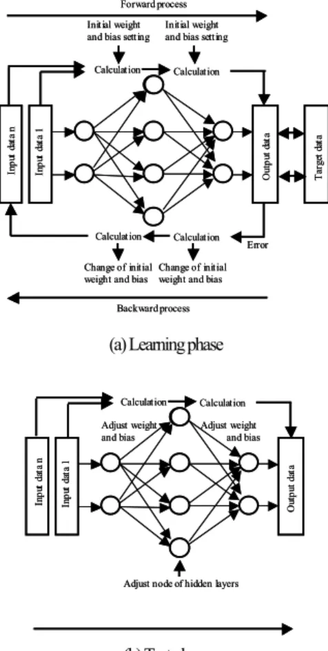
purpose of the neural network. The output layer produces the calculated output vectors corresponding to the solution. BPNN performs in two phases; learning (training) phase and testing (or validation) phase. During learning of the network, as in Fig. 3 (a), data is processed through the input layer to hidden layer, until it reaches the output layer, as is called forward process. In this layer, the output is compared to the targeted values (the "true" output). The difference or error between both is processed back through the network, as is called backward process, updating the individual weights of the connections and the biases of the individual neurons. The input and output data are mostly represented as vectors called training pairs. Each path through the entire training pattern is called a cycle or epoch. The process is then repeated as many epochs as needed until the error within the user specified goal is reached successfully. The process as mentioned above is repeated for all the training pairs in the dataset, until the network error converged to a threshold minimum defined by a corresponding sum square error function. Testing phase is a calculation process that is undertaken after training has been completed, as shown in Fig. 3 (b). In order to perform a BPNN analysis, one needs to be aware of several parameters and operations associated with network training (Hagazy et al., 1994).

Initial weight and bias setting

Calculation Calculation

Error Calculation Calculation

Change of initial weight and bias Change of initial weight and bias

Input data 1

Input data n Output data

Forward process

Backward process

Target data

Initial weight and bias setting

Error Calculation Calculation

Change of initial weight and bias Change of initial weight and bias

Input data 1

Forward process

Backward process

Target data

(a) Learning phase

Adjust weight and bias

Input data 1

Adjust weight 　　　　and bias

Adjust node of hidden layers Adjust weight

and bias

Input data 1

Adjust weight 　　　　and bias

Adjust node of hidden layers

(b) Test phase

Fig. 3. Learning and testing phase in neural network system

They are database size and partitioning, data preprocessing, balancing, data normalization, input / output representation, network weight initialization, BPNN learning rate and momentum coefficient,

transfer function, convergence criteria, number of training cycles, training modes, hidden layer size and parameter optimization so on (Basheer, 2000). Details of the BPNN algorithm are beyond the scope of this study and can be found in Hecht-Nielsen(1987).

Field study is performed by two NATM tunnel of the A and B Project in Japan. That this tunnel excavated through sandy layer under shallow depth and Auxiliary method is applied for face stabilization and water inflow control.

The standard tunnel cross section are given in Fig. 4. Supports reinforcements are rock bolt, shotcrete and steel support as show in Fig. 4. The excavation was conducted by the top heading and three bench cut method. Factors affecting tunnel behavior can be grouped into four major categories as show in Fig. 5.

Rockboltφ22mm

Bottom level

Lining 30cm Shotcrete 20cm Steel rib H150mm

Invert 45cm

R=7.35 R=4.35

0.40

2.60 R=9.79

2.50 2.90

Fig. 4. Details of tunnel cross section

Tunnel behavior

Tunnel geometry

Support condition and Auxiliary method Ground condition

Excavation condition Tunnel

behavior

Tunnel geometry

Support condition and Auxiliary method Ground condition

Excavation condition

Fig. 5. Four factors affecting tunnel behavior

4. ANN analysis with field database

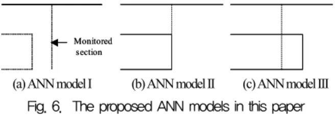
4.1 ANN model design and devolpment

The main focus of the ANN approach is to make the prediction model of tunnel behavior through existing data. The ANN maps input vectors onto output vectors. It can be trained to map given input vectors onto respective given output vectors referred to as desired output vector. The neural network in the input layer receives tunnel geometric, ground condition, excavation method and support system, as input values. Tunnel behaviors are to be determined from output values. In this paper, applied ANN analyses are summarized as following three conditions ; 1) ANN analysis I is prediction of tunnel behavior using acquired data before construction, 2) ANN analysis II is prediction of tunnel behavior using data acquired when the tunnel

(4)

face arrives at monitored section, and 3) ANN analysis III is prediction of Tunnel behavior using data acquired when the tunnel face is 1D away from the monitored section as shown in Fig.6.

Monitored section Monitored

section

(a) ANN model I (b) ANN model II (c) ANN model III Fig. 6. The proposed ANN models in this paper

Model input parameters are tunnel overburden, ground condition, excavation method, support condition, auxiliary method. And, output parameters of model are tunnel behavior in final excavation.

Table 1. Description of input an output parameter in ANN model I

Category Parameter items ANN

model I-1 ANN model I-2

ANN model I-3

ANN model I-4

Tunnel geometrics Overburden - Input Input Input Input

clay Input Input Input Input

sand Input Input Input Input

alt. of strata Input Input Input Input Unconsilidated

ground type - Input Input Input Input

Excavation method Top Heading and

Three bench cut method - Input Input Input Input

Shotcret - Input

rock bolt(length) - Input

rock bolt(number) - Input

H-steel - Input

Forepoling - Input Input Input

Steel pipe forepiling - Input Input Input

diameter × × Input Input

Length × × Input Input

number × × Input Input

construction

degree × × Input Input

Face bolt - Input Input

Face shotcrete - Input Input

Footing reinforcement bolt - Input Input Input Input

Crown - × × × ×

Convergence - × × × ×

Foot settlement - × × × ×

Crown - Output Output Output Output

Convergence - Output Output Output Output

Foot settlement - Output Output Output Output

Auxiliary method

Steel pipe forepiling specification

Tunnel behavior in final excavation Initial tunnel

behavior information Ground condition

Input Ground type

Input Support condition

Input

Input Input

Input

Table 2. Description of input an output parameter in ANN model II and III

Category Parameter items ANN

model II-1 ANN model II-

ANN model II-3

ANN model II-4

ANN model III-1

Tunnel geometrics Overburden - Input Input Input Input Input

clay Input Input Input Input Input

sand Input Input Input Input Input

alt. of strata Input Input Input Input Input Unconsilidated

ground type - Input Input Input Input Input

Excavation method Top Heading and

Three bench cut method - Input Input Input Input Input

Shotcret - Input

rock bolt(length) - Input

rock bolt(number) - Input

H-steel - Input

Forepoling - Input Input Input

Steel pipe forepiling - Input Input Input

diameter × × Input Input ×

Length × × Input Input ×

number × × Input Input ×

construction

degree × × Input Input ×

Face bolt - Input Input

Face shotcrete - Input Input

Footing reinforcement bolt - Input Input Input Input Input

Crown - × × × × Input

Convergence - × × × × Input

Foot settlement - × × × × Input

Crown - Output Output Output Output Output

Convergence - Output Output Output Output Output

Foot settlement - Output Output Output Output Output

Input

Input Input

Input

Input Input

Input Input Ground type

Input Ground condition

Input Input

Face estimation -

Support condition

Auxiliary method

Steel pipe forepiling specification

Tunnel behavior in final excavation

Initial tunnel behavior information

Ground condition in the tunnel used for neural network input are divided into three categories: (1) ground type around tunnel face, (2) the existence of unconsolidated soil and (3) one face record rating of the total geological at the tunnel. Geology type around tunnel face is divided into clay, sandy and alt. of strata. The rating of geology

characteristic at the tunnel face is calculated as according to the Japan standard specifications. The categories of 'excavation method' are divided into two categories: bench cut and three bench cut method.

Support conditions are selected in four factors as length and number of rock bolt, shotcrete and Steel beam type. Auxiliary reinforcements were especially considered because NATM tunneling method was commonly used NATM construction in non-stability ground. Five auxiliary reinforcement techniques, forepoling, steel pipe forepiling, face bolt, face shotcrete and footing reinforcement, were major methods as a countermeasure of settlement due to tunneling in Japan.

Details of input and output parameters of ANN analysis and various models are shown in Tables 1 and 2.

In ANN analysis I, input parameters are tunnel overburden, initially investigated ground condition, excavation method, support condition and auxiliary method, as design stage. In model I-1, support condition used as the input parameters in the logical variables, which applied to case 1 and did not apply to case 0 in ANN analysis. The input parameters of forepoling and steel pipe forepiling were used as one input variable, which was applied forepoling used as 0 and steel pipe forepiling used as 1. Input variables of steel pipe forepiling specification were not used in ANN analysis. In model I-2, the input parameters of forepoling and steel pipe forepiling were used as two input variable. In model I-3, steel pipe forepiling specifications were used as four variables in ANN analysis. In model I-4, support conditions were used as four input variable. Input parameters of ANN analysis model II included the face rating with ANN analysis model I ones, as tunnel face arrival stage. In ANN analysis model III, input parameters included the initial measure data with the ANN analysis model II.

In this study, field data are obtained by two NATM tunnel in A Project. It is a common practice to divide available data into two subsets; training set to construct a neural network model, and an independent testing set to estimate model performance in the deployed environment. In data number, 55% of the dataset (102case) was used for training and 45% of the dataset (83cases) was used for testing of the ANN model. After data division, it is important to pre- process the data to a suitable form before they are brought in to an ANN making procedure. Pre-processing the data, such as scaling, is important to ensure that all variables receive equal attention during training. The output variables have to be scaled to be commensurate with the limits of the transfer functions used in the output layer.

Scaling the input variables is not necessary but is always recommended (Hassoum, 1993). Despite its versatility, BPNN often faces shape criticism about the high computation for net work training and failure to guarantee its convergence (Suwansawat and Einstein, 2006). Generally, there is no direction and precise method for determining the most appropriate architecture and parameters for the selection of ANN model, although some guide lines are proposed

(5)

(Hegazy et al., 1994). Trial and error method is the only way to arrive at a suitable learning rate, momentum, number of training cycle and the optimal numbers of hidden node or hidden layer with the criterion error (Neaupane and Adhikari, 2006). The development process of ANN model I is shown in Fig. 7.

ANN analysis most commonly used for finding optimum weights is BPNN algorithm (Basheer and Hajmeer, 2000). Back-propagation of errors is called an epoch. The iteration step corresponds to an epoch number. In this paper, the convergence criteria are set such that the learning process is terminated when either of the following two conditions ; 1) Number of training cycles (Epoch) becomes 400,000, and 2) Error of the network becomes less than 0.0001. Once the training of a model has been successfully accomplished, performance of the trained model is validated using the testing data, which have not been used as the part of model building process. Testing result is used for the selection of an optimal ANN model.

Start

ANN Architecture Number of hidden layer

1 layer Nodes in hidden layer

1.ANN model I-1 10,12,14,16,18,20 2. ANN model I-2 16,18,20,22 3.ANN model I-3

16,20,24,28,32 4. ANN model I-4 19,22,26,30,34,38

ANN Parameters Learning Rule

Delta-Rule Tran formation Function

Sigmoid function Learning Rate

0.01,0.1,0.2,0.3 Moment Rate

0.1, 0.3,0.5

Learning process

Optimal ANN architecture and parameters Data preparation

Data Precession

Testing process Start

ANN Architecture Number of hidden layer

1 layer Nodes in hidden layer

1.ANN model I-1 10,12,14,16,18,20 2. ANN model I-2 16,18,20,22 3.ANN model I-3

16,20,24,28,32 4. ANN model I-4 19,22,26,30,34,38

ANN Parameters Learning Rule

Delta-Rule Tran formation Function

Sigmoid function Learning Rate

0.01,0.1,0.2,0.3 Moment Rate

0.1, 0.3,0.5

Learning process

Optimal ANN architecture and parameters Data preparation

Data Precession

Testing process

Fig. 7. ANN model I development process

4.2 Result of ANN analysis

Prediction of tunnel deformations was performed by ANN analysis with field database for two tunnels. In order to obtain better performance of the ANN model, the ANN architecture was tested with various numbers of nodes per hidden layer, various learning and momentum rates. After ANN analysis many trials, the summary of training and testing results are illustrated in Table 3, 4 and 5. The results shown in Table 3, 4 and 5 represented the best performing network that can be achieved in the present study. The proposed analysis of ANN model I-1 is shown in Fig. 8.

Overburden Clay

Presupport system Support system

Sand

Exc. method Uncol. ground Alter of strata Ground

condition

Face bolt and shot.

Footing rein. bolt

Cro wn/Convergence /Foot settlement Overburden

Clay

Presupport system Support system

Sand

Exc. method Uncol. ground Alter of strata Ground

condition

Face bolt and shot.

Footing rein. bolt

Cro wn/Convergence /Foot settlement

Fig. 8. Studied ANN model I-1

Table 3. Learning and testing result in ANN Analysis I

Input Hidden Output Correlation RMSE Correlation RMSE

Crown 50000 10 12 1 0.3/0.5 0.92 8.05 0.84 8.49

Convergence 50000 10 20 1 0.01/0.1 0.80 5.48 0.83 5.05

Foot settlement 50000 10 12 1 0.3/0.5 0.87 11.95 0.86 9.86

Crown 50000 11 18 1 0.2/0.5 0.94 7.14 8.07 0.86

Convergence 50000 11 16 1 0.01/0.1 0.80 5.48 0.84 4.86

Foot settlement 50000 11 12 1 0.3/0.5 0.87 11.72 0.84 10.26

Crown 50000 16 24 1 0.3/0.5 0.94 7.07 0.86 7.98

Convergence 50000 16 20 1 0.01/0.1 0.81 5.33 0.83 5.08

Foot settlement 50000 16 32 1 0.3/0.1 0.88 11.59 0.85 9.99

Crown 50000 19 38 1 0.3/0.5 0.94 7.09 0.86 8.02

Convergence 50000 19 34 1 0.01/0.1 0.80 5.45 0.84 4.91

Foot settlement 50000 19 19 1 0.3/0.5 0.88 11.59 0.87 9.51

ANN model I-4

ANN structure Final

epoch

Learning Testing

ANN analysis model I

ANN model I-3

Learning rate/

Momentum ANN

model I-1 ANN model I-2

Table 4. Learning and testing result in ANN Analysis II

Crown 50000 11 16 1 0.1/0.3 0.94 6.74 0.90 6.90

Convergence 50000 11 12 1 0.1/0.1 0.87 4.58 0.82 5.21

Foot settlement 50000 11 14 1 0.1/0.1 0.91 9.76 0.94 6.35

Crown 50000 12 20 1 0.1/0.3 0.94 6.95 0.90 6.82

Convergence 50000 12 16 1 0.01/0.1 0.81 5.41 0.83 5.08

Foot settlement 50000 12 20 1 0.1/0.5 0.92 9.15 0.93 6.70

Crown 50000 17 34 1 0.1/0.1 0.95 6.46 0.90 6.76

Convergence 50000 17 30 1 0.01/0.1 0.81 5.38 0.82 5.24

Foot settlement 50000 17 22 1 0.1/0.1 0.92 9.61 0.95 5.59

Crown 50000 20 20 1 0.1/0.3 0.94 7.09 0.91 6.66

Convergence 50000 20 36 1 0.01/0.1 0.80 5.45 0.83 5.10

Foot settlement 50000 20 28 1 0.1/0.1 0.91 9.75 0.95 5.66

Learning Testing

ANN analysis model II

ANN model II-3

Learning rate/

Momentum ANN

model II-1 ANN model II-2

ANN model II-4

ANN structure Final

epoch

Table 5. Learning and testing result in ANN Analysis III

Crown 50000 12 14 1 0.3/0.5 0.99 3.57 0.93 6.57

Convergence 50000 12 22 1 0.01/0.1 0.92 3.66 0.90 4.00

Foot settlement 50000 12 18 1 0.1/0.1 0.97 4.88 0.95 4.78

ANN model III-1

Final epoch

ANN analysis model III Learning rate/

Momentum

Learning Testing

ANN structure

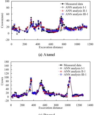
Training and testing results are plotted in Fig. 9 in ANN model I-1, II-1 and III-1. As see in the figure, the neural network model provided good prediction in agreement with measured settlements and its overall performance was much better. ANN analysis III-1 gave the good prediction accuracy compared with ANN analyses I-1 and II-1.

-20 0 20 40 60 80 100

0 200 400 600 800 1000 1200

Excavation distance

Crown(mm)

Measured data ANN analysis I-1 ANN analysis II-1 ANN analysis III-1

(a) A tunnel

-20 0 20 40 60 80 100 120 140 160 180

0 200 400 600 800 1000 1200 1400

Excavation distance

Crown

Measured data ANN analysis I-1 ANN analysis II-1 ANN analysis III-1

(a) B tunnel

Fig. 9. A measured and predicted results of crown settlement due to excavation length

(6)

5. ANN analysis with FEM database

5.1 Making ANN model

In making an optimized ANN model for parameter identification, measured displacements are input into a model, which outputs linear or nonlinear material properties, as depicted in Fig.10. A trained ANN model has the potential to provide accurate output from input data.

Once the ANN determines material properties, an FEM simulation can be performed for prediction of tunneling-induced deformation for following excavation stages.

Measured data

Input layer Hiddden layer

Output layer E Ko Δr β Design parameter

1 2 3

1 2

i j

1

Output Input

ANN Model Measured data

Input layer Hiddden layer

Output layer E Ko Δr β Design parameter

1 2 3

1 2

i j

1

Output Input

ANN Model

Fig.10 Fundamental flow of actions.

Two different timings, T1 and T2, are chosen for setting up ANN models for respective purposes, as described before. Firstly at T1, key parameters are Young’s modulus E and horizontal stress ratio K0. An ANN model set up is possible such that measured displacements are input into a model, and E, K0 are output simultaneously.

However, this set up was found to have some difficulty to obtain those output parameters with high accuracy. Trial and error investigation later revealed that a two-step approach is better. That is that the first ANN, Model-1, is set up such that measured displacement are input to define E only . The second ANN, Model-2, also uses the same measured displacement and the newly determined E as input data to define K0 . These two models, Model-1 and Model- 2 are defined at T1, the arrival of top heading face, as shown in Fig.11(a).

U₁ E

U_n E

U₁ U_n

U₁ U_n E

K₀ U₁

U_n E

K₀

Model-1 for E Model-2 for K0

(a) Two ANN models to be established for T1.

β U_n

E K₀

β U_n

E K₀ U_n E K₀

Δγ U_n

E K₀

β

Δγ U_n

E K₀

β

Model-3 for β Model-4 for Δγ (b) Two ANN models to be established for T2. Fig.11 ANN structures of the four models considered.

A similar two-step approach is also employed at the second timing, T2, which is defined at the completion of the top heading excavation., as shown in Fig.11(b). Model-3 uses measured displacements, E and K0 as input, to determine β which indicates ratio of dropped cohesion and friction angle to their original values. The last ANN model, Model-4, uses the measured displacement, E, K0 and β, to define the last key parameter Δγ which indicates strain increment during which strength parameters drop from original to residual values. By this strategy, two key parameters controlling elastic behavior of the ground can be determined at the arrival of top heading face. Other two parameters controlling nonlinear behavior can be determined when the top heading excavation is completed. A full set of linear and nonlinear parameters become available then to perform predictive analyses for remaining sequence of tunnel excavation.

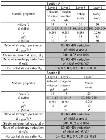
Table 6 Materials value used to generate FEM database.

Layer 1 Layer 2 Layer 3 Layer 4 Takadate

volcanic ash

Takadate volcanic ash

Noheji sandy

r(kN/m³) 14 18 20 20

E (MPa) 5, 10, 15 5, 10, 15 80, 160, 240 100, 200, 300

ν 0.286 0.286 0.286 0.286

φ(⁰) 0 0 35 35

c (MPa) 30 45 30 50

Ratio of strength parameter, β_c,φ(0)(%) Strain incremental ratio, Δγ Ratio of anisotropy reduction,

β m(%) Horizontal stress ratio, K₀

Layer 1 Layer 2 Takadate

volcanic ash

Tengutai volcanic ash

r(kN/m³) 14 18

E (MPa) 5, 10, 15 5, 10, 15

ν 0.286 0.286

φ(⁰) 30 45

c (MPa) 0 0

Ratio of strength parameter, β_c,_φ(0)(%) Strain incremental ratio, Δγ Ratio of anisotropy reduction,

;Selected value for FEM database Material properties

0.4, 0.5, 0.6, 0.7, 0.8, 0.9, 0.98

0.4, 0.5, 0.6, 0.7, 0.8, 0.9, 0.98 Material properties

Layer 3 Noheji sandy 20 80, 160, 240

0.286 30 35

80, 60, 40% reduction of initial m(=E/G) 80, 60, 40% reduction

of initial c and φ 0.01, 0.02 and 0.04 Section B

Section A

80, 60, 40% reduction of initial c and φ 0.01, 0.02 and 0.04 80, 60, 40% reduction

of initial m(=E/G)

For database generation by parametric FEM analyses, selection of key parameter values was conducted in such a way that the past records from relevant construction or of the lab test results were reflected in the minimum and maximum values of these parameters.

Table 6 shows the materials properties used for FEM database. Those parameters for which multiple variations were employed are shown by gray hatch. For example, three different values, namely 80, 60 and 40%, were used for β. Like wise, parameters Δγ, βm (ratio of mr to its original value mi) and K0 had 3, 3 and 7 different values. All possible combination of these variables led to 189 patterns (3×3×3×7) of

(7)

analyses, the results of which are to form the database.

The numbers of analysis cases for Sections A and B in learning and testing processes are shown in Table 7.

Table 7 Number of analysis cases for database generation. Section A Section B

Learning 189 189

Testing 28 35

Surface settlement 7point

Horizontal displacement 14point Subsurface settlement 10Point Surface settlement 7point

Horizontal displacement 14point Subsurface settlement 10Point

Fig.12 Measurement points for Section A.

Fig.12 shows the measurement point, as input parameter of ANN analysis. For both cross sections, E and K0 are determined using measured displacements at the arrival of the top heading; and β and Δγ are determined using measured displacements at the completion of the top heading of the tunnel. Details of input and output parameters of ANN models are shown in Table 8.

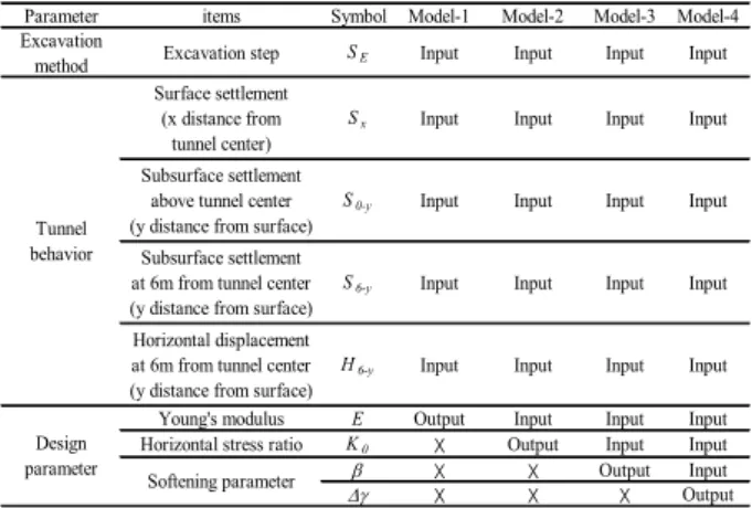
Table 8 Description of input and output parameter in ANN model for Section A.

Parameter items Symbol Model-1 Model-2 Model-3 Model-4

Excavation

method Excavation step S_E Input Input Input Input

Surface settlement (x distance from

tunnel center)

S_x Input Input Input Input

Subsurface settlement above tunnel center (y distance from surface)

S_0-y Input Input Input Input

Subsurface settlement at 6m from tunnel center (y distance from surface)

S6-y Input Input Input Input

Horizontal displacement at 6m from tunnel center (y distance from surface)

H6-y Input Input Input Input

Young's modulus E Output Input Input Input

Horizontal stress ratio K0 Ｘ Output Input Input

β ＸＸ Output Input

Δγ ＸＸＸ Output

Softening parameter Tunnel

behavior

Design parameter

5.2 Results of making ANNs

Firstly, parameter identification of E and K0 was performed initially at the timing of “top heading arrival”, assuming an elastic ground behavior. Secondly, β and Δγ, two most influential parameters characterizing nonlinear softening behavior, were determined by measured data after “top heading completion”. In order to obtain better performance of the ANN model, the ANN architecture was

tested with various numbers of nodes per hidden layer, various learning and momentum rates. Despite of learning data being adequately prepared, it is known that quality of an ANN varies depending on chosen network architecture and learning environments.

In addition, ANN learning process should be carefully carried out to guarantee generality for further application. After trying many learning and testing procedures, optimal architectures of ANN as well as adopted learning parameters were chosen, that are summarized in Table 9. The results shown in Table 9 represent the best performing network that was achieved in the present study.

Table 9 Learning and testing results.

Model-1 Model-2 Model-3 Model-4

E K0 β ⊿γ

Learning rule Delta rule Delta rule Delta rule Delta rule Transformation function Sigmoid Sigmoid Sigmoid Sigmoid

Structure 32-32-1 33-73-1 34-90-1 35-59-1

Learning rate 0.3 0.01 0.01 0.1

Momentum rate 0.9 0.9 0.1 0.9

Final sys. error 0.019 0.019 0.494 0.019

Final epoch(cycles) 18 2130 40000 40000

Learning RMSE 4.761 0.018 0.066 0.001

Testing RMSE 5.271 0.012 0.054 0.003

Learning R² 0.997 0.996 0.913 0.998

Testing R² 0.996 0.997 0.931 0.973

Model-1 Model-2 Model-3 Model-4

E K0 β ⊿γ

Learning rule Delta rule Delta rule Delta rule Delta rule Transformation function Sigmoid Sigmoid Sigmoid Sigmoid

Structure 16-16-1 17-25-1 18-18-1 19-27-1

Learning rate 0.1 0.1 0.3 0.01

Momentum rate 0.1 0.5 0.1 0.5

Final system error 0.018 0.019 0.534 0.112

Final epoch(cycles) 52 883 40000 40000

Learning RMSE 4.679 0.018 0.069 0.002

Testing RMSE 6.138 0.016 0.062 0.005

Learning R² 0.999 0.996 0.906 0.986

Testing R² 0.999 0.996 0.899 0.942

Model

0.0 50.0 100.0 150.0 200.0 250.0 300.0

0.0 50.0 100.0 150.0 200.0 250.0 300.0 True Values

Computed Values

Learning Testing

(a) E

0.00 0.01 0.02 0.03 0.04 0.05

True Values

Computed Values

Learning Testing

(b) Δγ

Fig. 13 Comparison of true value and computed one by the selected ANN model in Section A.

(8)

Fig. 13 shows comparison of true values and computed ones using the selected ANN models for Sections A and B. As for the results for Section A, a strong correlation between the true and computed values is seen for elastic parameters, E and Δγ.

In contrast, some scattering is seen especially for β reflecting the relative difficulty in estimating a parameter concerned with nonlinear behavior.

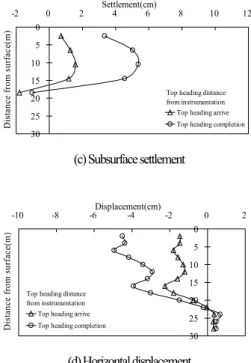
Fig. 14 shows the measured displacement at top heading arrival and completion for Section A.

-20 -16 -12 -8 -4 0

0 10 20 30 40

Distance from tunnel center(m)

Subsidence (mm)

Top heading arrive Top heading completion Top heading distance from instrumentation

(a) Subsidence

0 2 4 6 8 10 12

-1 0 1 2 3 4 5

Settlement(cm)

Distance from surface(m)

(b) Subsurface settlement above tunnel

0 5 10 15 20 25 30

-2 0 2 Settlement(cm)4 6 8 10 12

(c) Subsurface settlement

0 5 10 15 20 25 30

-10 -8 -6Displacement(cm)-4 -2 0 2

(d) Horizontal displacement

Fig. 14 Measured data in the top heading stage.

Measured data were used as input data for back analyses based on ANN model. Tables 10 show the parameters identified by the optimized ANN models. Strain softening analysis was then performed using identified parameters to simulate all excavation processes.

Table 10 Identified parameter value for Section A (*marked value).

Layer 1 Layer 2 Layer 3 Layer 4 Takadate

volcanic ash

Takadate volcanic

ash

Noheji sandy

r(kN/m³) 14 18 20 20

E (MPa) 14.3* 14.3* 229* 286*

ν 0.286 0.286 0.286 0.286

φ(⁰) 0 0 35 35

c (MPa) 30 45 30 50

Ration of strength parameter, β_c,φ(0)(%) Strain incremental ration, Δγ Ration of anisotropy reduction,

Section A

36*

0.01*

36*

Material properties

0.98*

0 3 6 9 12 15

0 5 Distance from tunnel center (m)10 15 20 25 30 35

Subsidence (mm)

Strain softening analysis

Measurement

(a) Surface settlement

(b) Maximum shear strain distribution at T4 (left) and I4 (right). Bright color near the tunnel wall shows strain greater than 1%.

Fig. 15 Comparison of measured and calculated displacement at invert stage for section A.

Figs.15 shows the comparison of the predicted and measured values in the subsidence settlement and the maximum shear strain distribution for the final stage (completion of invert).

6. Conclusion

The main objective of this thesis is to perform the deformation analysis in NATM tunnel by means of artificial neural network (ANN) and field database. The proposed methodology of using ANN technique in parameter identification problems works with

(9)

other engineering methods, such as nonlinear finite element analysis or field measurement conducted onsite. Since the direct source of information from which unknown parameters are determined is measured displacement, the parameters obtained have practical values. Once the network is trained, its running speed is very high, thereby reducing the total time consumed in the analysis. The proposed method based on ANN and field database offers a practical way for prediction final displacement of shallow NATM tunnel, enabling rational safety management scheme to be employed.

References

1) Basheer, I. A. and Hajmeer, M.: Artificial neural networks:

fundamentals, computing, design, and application, Journal of Micro-biological Methods, 43, 3-31, 2000.

2) Hegazy, T., Fazio, P., Moselhi, O.: Developing Practical Neural Network Application using Back-Propagation. Microcomputers in Civil Engineering, 9, pp. 145-159, 1994.

3) Hassoum, M. H.:Fundamentals of artificial neural networks.

Cambridge MA : MIT. Press, 1995.

4) Hecht-Nielsen, R.: Kolmogorov's mapping neural network existence theorem, Proceedings of the first IEEE international conference on neural networks, San Diego CA, USA, 11-14, 1987.

5) Neaupane, K. M., Adhikari, N. R.: Prediction of tunneling-induced ground movement with the multi-layer perceptron, Tunnelling an Underground Space Technology, 21, 151-159, 2006.

6) Rumelhart D. E, Hinton G. E. and Williams R. F.: Learning internal representation by error propagation. In : Rumelhart DE, McClelland JL, dedtors. Parallel distributed processing, vol. 1, 318- 362, 1986.

7) Rumelhart, D. E., Durbin, R.: Golden, R. and Chauvin, Y.:

Backpropa -gation: the basic theory. In : Rumelhart, D.E., Yves,C.

(Eds.), Backpropagation: Theory, Architecture, and Applications, Lawrence Eribaum, Nj, 1-34, 1995.

8) Suwansawat, S., Einstein, H. H.: Artificial neural networks for predicting the maximum surface settlement caused by EPB shield tunneling. Tunnelling and Underground Space Technology, 21, 133-150, 2006.