Bayes tests of independence for contingency tables from small areas

Bayes tests of independence for contingency tables from small areas

Aejung Jo ¹ · Dal Ho Kim ²

12 Department of Statistics, Kyungpook National University

Received 9 October 2016, revised 30 October 2016, accepted 1 November 2016

Abstract

In this paper we study pooling effects in Bayesian testing procedures of indepen- dence for contingency tables from small areas. In small area estimation setup, we typi- cally use a hierarchical Bayesian model for borrowing strength across small areas. This techniques of borrowing strength in small area estimation is used to construct a Bayes test of independence for contingency tables from small areas. In specific, we consider the methods of direct or indirect pooling in multinomial models through Dirichlet pri- ors. We use the Bayes factor (or equivalently the ratio of the marginal likelihoods) to construct the Bayes test, and the marginal density is obtained by integrating the joint density function over all parameters. The Bayes test is computed by performing a Monte Carlo integration based on the method proposed by Nandram and Kim (2002).

Keywords: Bayes factor, Dirichlet priors, Gibbs sampler, pooling, small areas.

1. Introduction

In many surveys, there are several small areas and a contingency table is constructed for each area. We consider a hierarchical Dirichlet-multinomial model to analyze the counts from these small areas. Our concern is to perform a test of independence which is competitive to the chi-square test for a single table. We follow a Bayesian inferential procedure so that appropriate priors are needed.

Statistical inference for small areas requires considerable care because the sample sizes for small areas are usually very small. To solve this problem, we use a hierarchical model which is to borrow strength some information from the neighboring areas. In this paper, we use the hierarchical Bayesian model to study the pooling effects in Bayesian tests of independence for contingency tables from small areas.

There are several literatures on methods for pooling of data. Malec and Sedransk (1992) developed a Bayesian procedure for estimation of the means for the specified experiments among a set of seemingly similar experiments. The proposed flexible prior distribution allows the intensity and nature of the pooling to be influenced by the sample data. Evans and Sedransk (1999) proposed an alternative Bayesian model with covariates that is more flexible.

1

Ph.D. candidate, Department of Statistics, Kyungpook National University, Daegu 702-701, Korea

2

Corresponding author: Professor, Department of Statistics, Kyungpook National University, Daegu

702-701, Korea. E-mail: [email protected]

Evans and Sedransk (2003) provided a fully Bayesian justification for the results in Malec and Sedransk.

There is a wide literature on Bayesian methods for analyzing data with contingency ta- bles. Agresti and Hitchcock (2005) surveyed Bayesian methods for categorical data analysis, with emphasis on contingency table analysis. The general concern with hierarchical Bayesian approach to contingency table analysis is how to handle the hyperparameters. In Dirichlet- multinomial model, Leonard (1977) made approximations when deriving the posterior to account for hyperparameter uncertainty. By contrast, Nandram (1998) used the Metropolis- Hastings algorithm to sample from the posterior distribution, rendering Leonard’s approx- imation unnecessary. Recently hierarchical Bayesian models in the contingency tables from small areas with nonresponses have been studied in Woo and Kim (2015, 2016).

In this paper, we will construct Bayesian tests of independence using a hierarchical multi- nomial model with Dirichlet priors. We will investigate the pooling effects in Bayes factors through the three different types of pooling strategies for Dirichlet priors; no pooling, com- plete pooling and adaptive pooling. In Section 2, we introduce the hierarchical Bayesian models under the three different types of pooling strategies for the test of independence.

Then we obtain the corresponding three Bayes factors using the marginal likelihoods. In Section 3, we present the results of numerical study with some simulated data. Finally, we provide some discussion and concluding remarks in Section 4.

2. Hierarchical Bayesian models

2.1. General models

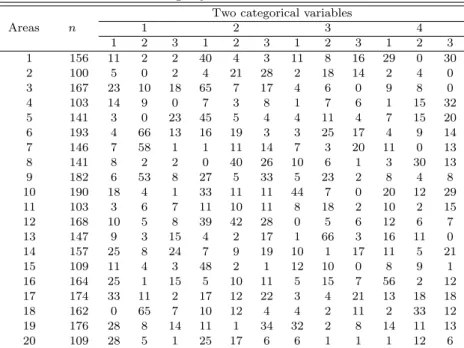
For the sth area of S small areas, we consider the r × c contingency tables with cell counts, n _sjk , which are the responses for the kth column and jth row in the sth area. Let π _sjk denote the corresponding probabilities of each unit cell in the sth area. When p _sj and q _sk are marginal probabilities for each column and each row in the sth area, the independence models have π _sjk = p _sj q _sk , j = 1, · · · , r, k = 1, · · · , c, where P r

j=1 p _sj = 1 and P c

k=1 p _sk = 1 for s = 1, · · · , S. Let n _si , i = 1, · · · , I (= rc) denote the cell counts for the sth area and π _si denote the corresponding probabilities of each area. We assume that

n _s |π _s ^ind ∼ Multinimial(n _s , π _s ), s = 1, · · · , S (2.1) where n _s = (n _s1 , · · · , n _sI ) for s = 1, · · · , S is the vector of responses with n _s = P I

i=1 n _si , total sum of responses, and π s = (π s1 , · · · , π sI ) is the corresponding probability vector of each area with P I

i=1 π si = 1. Here I is denoted by the number of cells for the table corresponding to each area.

Now we consider three types of pooling strategies for the general model (2.1).

1) No pooling, π s

iid ∼ Dirichlet(1), s = 1, · · · , S;

2) Complete pooling, ˜ π ∼ Dirichlet(1) with π ₁ = · · · = π _S = ˜ π;

3) Adaptive pooling, π s

iid ∼ Dirichlet(µτ ), where µ = (µ ₁ , · · · , µ _K ), 0 ≤ µ _k ≤ 1, P K

k=1 µ _k = 1 and τ > 0 are hyperparameters

for Dirichlet distribution and are assumed to have the noninformative and proper prior

π(µ, τ ) = (K − 1)!/(1 + τ ) ² . This prior is very similar to a half-Cauchy prior and can pre- vent overestimation of scale parameters from our models. Recall that x|µ, τ ∼ Dirichlet(µτ ) has the density f (x|µ, τ ) = Q k

i=1 x ^µ _i

ⁱ

^{τ −1} /D(µτ ), 0 < x _i < 1, P k

i=1 x _i = 1 where D(µτ ) = Q k

i=1 Γ(µ i τ )/Γ(τ ), 0 < µ i < 1, τ > 0, is the Dirichlet function, also known as the multivari- ate Beta function.

Under no pooling, the joint density function for all variables is

π(n, π) =

S

Y

s=1

{f (n s |π s )π(π s )} =

S

Y

s=1

n n s ! Q I

i=1 n _si !

I

Y

i=1

π _si ⁿ

^si

(I − 1)! o ,

where n = (n 1 , · · · , n S ) and π = (π 1 , · · · , π S ). In no pooling, we could not obtain any information from prior distribution. For the marginal likelihood, we can use the posterior density of π _s given n _s ,

π s | n s

ind ∼ Dirichlet(n s + 1), s = 1, · · · , S.

So we obtain the marginal likelihood for the sth area,

f (n _s ) = n _s !(I − 1)!

Q I i=1 n _si !

Q I

i=1 Γ(n si + 1) Γ( P I

i=1 n _si + I) . Under complete pooling, the joint density function is

π(n, ˜ π) =

S

Y

s=1

{f (n s | ˜ π)}π( ˜ π) =

S

Y

s=1

n n s ! Q I

i=1 n si !

I

Y

i=1

˜ π ⁿ _i

^si

o

(I − 1)!

where ˜ π = (˜ π 1 , · · · , ˜ π I ). The parameter ˜ π is shared by the data in entire areas. Then we can calculate the marginal likelihood using the posterior density of ˜ π which is the Dirichlet distribution with parameter P S

s=1 n s + 1. Our marginal likelihood under complete-pooling is

f (n) = Q S

s=1 n s !(I − 1)!

Q S s=1

Q I i=1 n si !

Q S s=1

Q I

i=1 Γ(n si + 1) Γ( P S

s=1

P I

i=1 n si + I) where Γ(t) = R ∞

0 x ^t−1 e ^−x dx is the gamma function. In complete pooling, the data are tied by interested parameter ˜ π, so our marginal likelihood for entire areas is expressed in just one equation. The idea of complete-pooling can be a contrast to no-pooling case.

Under adaptive pooling, the joint density function for all variables is

π(n, π, µ, τ ) =

S

Y

s=1

n n _s ! Q I

i=1 n si !

I

Y

i=1

π _si ⁿ

^si

1 D(µτ )

I

Y

i=1

π _si ^µ

ⁱ

^{τ −1} o (I − 1)!

(1 + τ ) ² .

Here we need to know the posteriors for all parameters to be integrated out in the joint density function. The posterior density of π _s , s = 1 · · · , S under adaptive-pooling is

π _s | n s , µ, τ ^ind ∼ Dirichlet(n s + µτ ), s = 1, · · · , S;

π(µ, τ | n) ∝

S

Y

s=1

n Y ^I

i=1

D(n _s + µτ ) D(µτ )

o 1

(1 + τ ) ² .

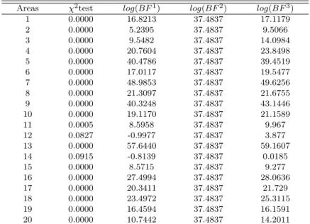
Each area has separate parameter vector π s for s = 1, · · · , S. However, the data in all areas is indirectly pooled by hyper-parameters µ and τ . Using these posteriors, we obtain the marginal likelihood

f (n s ) = (I − 1)!n s ! Q I

i=1 n si ! Z

µ Z

τ

D(µτ + n s )

D(µτ )(1 + τ ) ² dµdτ, s = 1 · · · , S.

For the computation of this marginal likelihood, we can use the method developed by Nan- dram and Kim (2002). They use an importance function which exploits the multiplication rule of probability, and is appropriate for any hierarchical model.

2.2. Independence models

Let n sjk , j = 1, · · · , r, k = 1, · · · , c, be the cell counts for jth row and kth column in sth area, s = 1, · · · , S with corresponding cell probability π sjk = p sj q sk where p sj = P c

k=1 π sjk

and q sk = P r

j=1 π sjk . We assume that

n _s |p _s , q _s ^ind ∼ Multinomial(n s , vec(p _s q ⁰ _s )), s = 1, . . . , S (2.2) where n s = (n s11 , · · · , n s1c , · · · , n sr1 , · · · , n src ), n s = P r

j=1

P c

k=1 n sjk , p _s = (p s1 , · · · , p sr ), q _s = (q s1 , · · · , q sc ), P r

j=1 p sj = 1, and P c

k=1 q sk = 1.

For the independence model (2.2), we consider no pooling p _s ^iid ∼ Dirichlet(1 p );

q _s ^iid ∼ Dirichlet(1 q ).

Under no pooling, the joint density function for all variables is π(n _s , p _s , q _s ) = n _s !

Q r j=1

Q c

k=1 n sjk !

r

Y

j=1 c

Y

k=1

(p _sj q _sk ) ⁿ

^sjk

(r − 1)!(c − 1)!, s = 1, . . . , S.

Then the marginal likelihood for the sth area is f (n s ) = (r − 1)!(c − 1)! n s !

Q r j=1

Q c

k=1 n _sjk ! Z

p

_s

r

Y

j=1

p ⁿ _sj

^sjk

dp _s Z

q

_s

c

Y

k=1

q _sk ⁿ

^sjk

dq _s .

Using the posterior distributions,

p _s | n ⁽¹⁾ _s ^ind ∼ Dirichlet(n ⁽¹⁾ _s + 1) and q _s | n ⁽²⁾ _s ^ind ∼ Dirichlet(n ⁽²⁾ _s + 1), where n ⁽¹⁾ s = (n ⁽¹⁾ _s1 , · · · , n ⁽¹⁾ sr ), n ⁽¹⁾ _sj = P c

k=1 n _sjk , j = 1, · · · , r, n ⁽²⁾ s = (n ⁽²⁾ _s1 , · · · , n ⁽²⁾ sc ), n ⁽²⁾ _sk = P r

j=1 n _sjk , k = 1, · · · , c, we obtain the marginal likelihood f (n _s ) = (r − 1)!(c − 1)! n _s !

Q r j=1

Q c

k=1 n sjk ! Q r

j=1 Γ(n ⁽¹⁾ _sj + 1) Q c

k=1 Γ(n ⁽²⁾ _sk + 1) Γ( P r

j=1 n ⁽¹⁾ _sj + r)Γ( P c

k=1 n ⁽²⁾ _sk + c)

.

Under no pooling, the Bayes factor (BF) of the general model versus the independence model for the sth area is

BF _s ¹ = (rc − 1)! Q r j=1

Q c

k=1 Γ(n sjk + 1)Γ( P r

j=1 n ⁽¹⁾ _sj + r)Γ( P c

k=1 n ⁽²⁾ _sk + c) (r − 1)!(c − 1)!Γ( P r

j=1

P c

k=1 n sjk + I) Q r

j=1 Γ(n ⁽¹⁾ _sj + 1) Q c

k=1 Γ(n ⁽²⁾ _sk + 1) .

Next, we consider complete pooling for the independence model, p ₁ = · · · = p _S = p ∼ Dirichlet(1 p );

q ₁ = · · · = q _S = q ∼ Dirichlet(1 q ),

where p = (p ₁ , · · · , p _r ), q = (q ₁ , · · · , q _c ). Under complete pooling, the joint density function for all variables is

π(n, p, q) =

S

Y

s=1

n s ! Q r

j=1

Q c

k=1 n sjk !

r

Y

j=1 c

Y

k=1

(p j q k ) ⁿ

^sjk

(r − 1)!(c − 1)!, s = 1, . . . , S.

Then the marginal likelihood is

f (n) = Z

p Z

q

S

Y

s=1

n _s ! Q r

j=1

Q c

k=1 n sjk !

r

Y

j=1 c

Y

k=1

(p j q k ) ⁿ

^sjk

(r − 1)!(c − 1)!dpdq.

Using the posterior distributions,

p | n ⁽¹⁾ ∼ Dirichlet(

S

X

s=1

n ⁽¹⁾ _s + 1) and q | n ⁽²⁾ ∼ Dirichlet(

S

X

s=1

n ⁽²⁾ _s + 1),

where n ⁽¹⁾ = (n ⁽¹⁾ ₁ , · · · , n ⁽¹⁾ _S ), n ⁽¹⁾ s = P c

k=1 n sjk , n ⁽²⁾ = (n ⁽²⁾ ₁ , · · · , n ⁽²⁾ _S ), n ⁽²⁾ s = P r

j=1 n sjk , we have the marginal density as follows.

f (n) = (r − 1)!(c − 1)! Q S s=1 s s ! Q S

s=1

Q r j=1

Q c

k=1 n sjk ! Q r

j=1 Γ( P S

s=1 n ⁽¹⁾ _sj + 1) Q c

k=1 Γ( P S

s=1 n ⁽²⁾ _sk + 1) Γ( P r

j=1

P S

s=1 n ⁽¹⁾ _sj + r)Γ( P c k=1

P S

s=1 n ⁽²⁾ _sk + c) .

Under complete-pooling, we obtain the Bayes factor of the general model versus the inde- pendence model for all areas,

BF ² = (rc − 1)! Q S s=1

Q I

i=1 Γ(n _si + 1)Γ( P r j=1

P S

s=1 n ⁽¹⁾ _sj + r)Γ( P c k=1

P S

s=1 n ⁽²⁾ _sk + c) (r −1)!(c −1)!Γ( P S

s=1

P I

i=1 n si +I) Q r

j=1 Γ( P S

s=1 n ⁽¹⁾ _sj +1) Q c

k=1 Γ( P S

s=1 n ⁽²⁾ _sk +1) ,

where n ⁽¹⁾ _sj = P c

k=1 n sjk , n ⁽²⁾ _sk = P r

j=1 n sjk . This Bayes factor is the same for all areas. It means that the all areas are regarded as strata with same characteristics in one grand area.

Under two pooling strategies, the Bayes factors are too much influenced by observed sample

data because the priors are noninformative. To complement this concern, we consider the

hierarchical Bayesian model under adaptive-pooling. In specific, adaptive pooling for the

independence model is given by

p _s ^iid ∼ Dirichlet(µ ₁ , τ 1 );

q _s ^iid ∼ Dirichlet(µ ₂ , τ 2 );

π(µ ₁ , τ 1 ) = (r − 1)!

(τ ₁ + 1) ² , π(µ ₂ , τ 2 ) = (c − 1)!

(τ ₂ + 1) ² , where µ ₁ = (µ 11 , · · · , µ 1r ), P r

j=1 µ 1j = 1, 0 < µ 1j < 1, j = 1, · · · , r, µ ₂ = (µ 21 , · · · , µ 2c ), P c

k=1 µ 2k = 1, 0 < µ 2k < 1, k = 1, · · · , c, τ 1 > 0, and τ 2 > 0. Under adaptive pooling, the joint density function for the sth area is

π(n s , p _s , q _s , µ ₁ , µ ₂ , τ 1 , τ 2 ) = n _s ! Q r

j=1

Q c

k=1 n sjk !

r

Y

j=1 c

Y

k=1

(p sj q sk ) ⁿ

^sjk

1 D(µ ₁ τ 1 )

r

Y

j=1

p ^µ _sj

^1j

^τ

¹

⁻¹

× 1

D(µ ₂ τ 2 )

c

Y

k=1

q ^µ _sk

^2k

^τ

²

⁻¹ (r − 1)!

(1 + τ 1 ) ²

(c − 1)!

(1 + τ 2 ) ² . In the joint density function, f (n _s | p _s , q _s ) is also rewritten as

f (n s |p _s q _s ) = Q r

j=1 n ⁽¹⁾ _sj Q c k=1 n ⁽²⁾ _sk n s ! Q r

j=1

Q c

k=1 n sjk ! f (n ⁽¹⁾ _s |p _s )f (n ⁽²⁾ _s |q ₂ ) where f (n ⁽¹⁾ s |p _s ) = _Q

_r

ⁿ

^s

^!

j=1

n

⁽¹⁾_sj

Q r

j=1 p ⁿ _sj

^sjk

and f (n ⁽²⁾ s |q ₂ ) = _Q

_c

ⁿ

^s

^!

k=1

n

⁽²⁾_sk

Q c

k=1 q _sk ⁿ

^sjk

for s = 1, · · · , S. Then we can calculate the marginal likelihood under adaptive pooling using the rewritten expression for f (n _s | p _s , q _s ). The marginal likelihood is

f (n _s ) = (r − 1)!(c − 1)!n _s ! Q r

j=1

Q c

k=1 n sjk !

Z Z Z Z D(µ ₁ τ ₁ + n ⁽¹⁾ s )D(µ ₂ τ ₂ + n ⁽²⁾ s )

D(µ ₁ τ 1 )D(µ ₂ τ 2 )(1 + τ 1 ) ² (1 + τ 2 ) ² dµ ₁ dτ ₁ dµ ₂ dτ ₂ . Hence the Bayes factor of the general model versus the independence model for the sth area under adaptive pooling is

BF _s ³ =

(rc − 1)! R R D( µ τ +n

_s

) D( µ τ +1)

²

dµdτ (r − 1)!(c − 1)! R R R R D( µ

₁

τ

₁

+n

⁽¹⁾_s

)D( µ

₂

τ

₂

+n

⁽²⁾_s

)

D( µ

₁

τ

1

)D( µ

₂

τ

2

)(τ

1

+1)

²

(τ

2

+1)

²

dµ ₁ dτ ₁ dµ ₂ dτ ₂ .

3. Numerical study

Our interest is to investigate the pooling effects by comparing Bayes factors through

the three different types of pooling strategies; no pooling, complete pooling and adaptive

pooling. For the comparative study, we generate the simulated data which construct the

two categorical variables. Specifically, we generated the data such that the one variable is

divided into 3 levels, while the other is composed of 4 categories in 20 areas. So we have 3 × 4

contingency tables from 20 areas. Here the response probabilities are taken from uniform

Dirichlet distribution.

Table 3.1 Contingency tables from the simulated data

Areas n

Two categorical variables

1 2 3 4

1 2 3 1 2 3 1 2 3 1 2 3

1 156 11 2 2 40 4 3 11 8 16 29 0 30

2 100 5 0 2 4 21 28 2 18 14 2 4 0

3 167 23 10 18 65 7 17 4 6 0 9 8 0

4 103 14 9 0 7 3 8 1 7 6 1 15 32

5 141 3 0 23 45 5 4 4 11 4 7 15 20

6 193 4 66 13 16 19 3 3 25 17 4 9 14

7 146 7 58 1 1 11 14 7 3 20 11 0 13

8 141 8 2 2 0 40 26 10 6 1 3 30 13

9 182 6 53 8 27 5 33 5 23 2 8 4 8

10 190 18 4 1 33 11 11 44 7 0 20 12 29

11 103 3 6 7 11 10 11 8 18 2 10 2 15

12 168 10 5 8 39 42 28 0 5 6 12 6 7

13 147 9 3 15 4 2 17 1 66 3 16 11 0

14 157 25 8 24 7 9 19 10 1 17 11 5 21

15 109 11 4 3 48 2 1 12 10 0 8 9 1

16 164 25 1 15 5 10 11 5 15 7 56 2 12

17 174 33 11 2 17 12 22 3 4 21 13 18 18

18 162 0 65 7 10 12 4 4 2 11 2 33 12

19 176 28 8 14 11 1 34 32 2 8 14 11 13

20 109 28 5 1 25 17 6 6 1 1 1 12 6

We consider three Bayes tests of independence as well as classical χ ² test. The χ ² test is done for the single table in each area and so it does not allow for any pooling of data from different areas. Bayes test under no pooling is a direct Bayes test which uses only data from each area. However, Bayes test under complete pooling regards all areas as one grand area.

Moreover, Bayes test under adaptive pooling is a indirect Bayes test which uses the data in all areas indirectly pooled by hyperparameters. Table 3.1 shows that the simulated counts in each area (a row of the table) are formed into a 3 × 4 contingency table.

Strictly speaking while the p-value can be used to provide evidence for the alternative, the Bayes factor can be used to provide evidence of either the null hypothesis or the alternative hypothesis over the other. If the log(BF ) is in (0, 1) or the p-value is in (.05, .10) we get borderline evidence against the null hypothesis. If the log(BF ) is in (1, 3) or the p-value is in (.025, .05), we get positive evidence against the null hypothesis. If the log(BF ) is in (3, 5) or the p-value is in (.01, .025), we get strong evidence against the null hypothesis. If the log(BF ) is greater than 5 or the p-value is in (.000, .010), we get very strong evidence against the null hypothesis; see Kass and Raftery (1995).

In Table 3.2, we compare the log(BF ) values of three Bayes tests with the p-values of the

classical χ ² test. The classical χ ² test is comparable to both Bayes test under no pooling

and Bayes test under adaptive pooling. But Bayes test under complete pooling provides

very strong evidence against the null hypothesis in all areas which might lead misleading

in inference. There are some areas in which the χ ² test and Bayes test under no pooling

provide same inferences, but Bayes test under no pooling and Bayes test under adaptive

pooling lead to different inference.

Table 3.2 Comparisons of the χ

²

test and three Bayes tests Areas χ

²

test log(BF

¹

) log(BF

²

) log(BF

³

)

1 0.0000 16.8213 37.4837 17.1179

2 0.0000 5.2395 37.4837 9.5066

3 0.0000 9.5482 37.4837 14.0984

4 0.0000 20.7604 37.4837 23.8498

5 0.0000 40.4786 37.4837 39.4519

6 0.0000 17.0117 37.4837 19.5477

7 0.0000 48.9853 37.4837 49.6256

8 0.0000 21.3097 37.4837 21.6755

9 0.0000 40.3248 37.4837 43.1446

10 0.0000 19.1170 37.4837 21.1589

11 0.0005 8.5958 37.4837 9.967

12 0.0827 -0.9977 37.4837 3.877

13 0.0000 57.6440 37.4837 59.1607

14 0.0915 -0.8139 37.4837 0.0185

15 0.0000 8.5715 37.4837 9.277

16 0.0000 27.4994 37.4837 28.0636

17 0.0000 20.3411 37.4837 21.729

18 0.0000 23.4972 37.4837 25.3115

19 0.0000 16.4594 37.4837 16.1591

20 0.0000 10.7442 37.4837 14.2011

We have monitored the convergence of Gibbs sampler using Geweke’s test and trace plots.

It turns out that our Gibbs sampler is enough to have convergence to get random samples based on some diagnostic measures.

Table 3.3 Geweke’s statistic for convergence diagnostic in Gibbs sampler General model

µ

1

µ

2

µ

3

µ

4

µ

5

µ

6

Statistics -0.5503 0.4695 1.9387 -0.0118 0.4447 -1.4995 p-value 0.5821 0.6387 0.0525 0.9906 0.6565 0.1337

µ

7

µ

8

µ

9

µ

10

µ

11

µ

12

Statistics -0.6491 0.5523 2.1683 -0.2583 -1.8313 0.103 p-value 0.5163 0.5807 0.0301 0.7962 0.0671 0.9179 Independence model

µ

11

µ

12

µ

13

Statistics -0.6962 -0.1775 1.3423 p-value 0.4863 0.8591 0.1795

µ

21

µ

22

µ

23

µ

24

Statistics 2.2492 -0.6979 -0.9235 -1.1826 p-value 0.0245 0.4853 0.3557 0.2370

Figure 3.1 Trace plots of µ

1

in Gibbs sampler

4. Concluding remarks

This article has presented Bayes factors for the test of independence for contingency tables from small areas. To obtain the test statistics, we have constructed the hierarchical Bayesian model with Dirichlet priors. In both no pooling and complete pooling, the data are directly pooled by probability parameters of Multinomial distribution. On the contrary to this, the adaptive pooling is assumed that the data are pooled indirectly by hyper-parameters in Dirichlet prior. Then we compare the Bayes factors with the χ ² test. We generate the data from uniform Dirichlet distribution and analyze the simulated data. As a result, the adaptive pooling seems to provide the better inference among three pooling strategies. By using indirect pooling method, we can calculate better test statistic which allows borrowing information from similar areas like in small area estimation.

References

Agresti, A. and Hitchcock, D. B. (2005). Bayesian inference for categorical data analysis. Statistical Methods and Applications, 14, 297-330.

Evans, R. and Sedransk, J. (1999). Methodoloty for pooling subpopulation regressions when sample sizes are small and there is uncertainty about which subpopulations are similar. Statistica Sinica, 9, 345-359.

Evans, R. and Sedransk, J. (2003). Bayesian methodology for combining the results from different ex- periments when the specifications for pooling are uncertain: II. Journal of Statiatical Planning and Inference, 111, 95-100.

Kass, R. E. and Raftery, A. E. (1995). Bayes factor. Journal of the American Statistical Association, 90, 773-795.

Leonard, T. (1977). Bayes simultaneous estimation for several multinomial distributions. Communications in Statistics: Theory and Methods, 6, 619-630.

Malec, D. and Sedransk, J. (1992). Bayesian methodology for combining the results from different experi- ments when the specifications for pooling are uncertain. Biometrika, 79, 593-601.

Nandram, B. (1998). A Bayesian analysis of the three-stage hierarchical multinomial model. Journal of Statistical Computation and Simulation, 61, 97-112.

Nandram, B. and Kim, H. (2002). Marginal likelihood for a class of Bayesian generalized linear models.

Journal of Statistical Computation and Simulation, 72, 319-340.

Woo, N. and Kim, D. H. (2015). A Bayesian uncertainty analysis for nonignorable nonresponse in two-way contingency table. Journal of the Korean Data & Information Science Society, 26, 1547-1555.

Woo, N. and Kim, D. H. (2016). A Bayesian model for two-way contingency tables with nonignorable

nonresponse from small areas. Journal of the Korean Data & Information Science Society, 27, 245-

254.