IEG 환경지질연구정보센터

Geosciences Journal

Vol. 11, No. 4, p. 387−396, December 2007

Hydraulic conductivity and mechanical stiffness tensors for variably saturated true anisotropic intact rock matrices, joints, joint sets, and jointed rock masses

ABSTRACT: A series of global hydraulic conductivity and mechanical stiffness tensors for variably saturated true anisotropic intact rock matrices, joints, joint sets, and jointed rock masses is formulated to expand the fully coupled poroelastic governing equations presented by Kim (2004) for groundwater flow and solid skeleton deformation in porous geologic media to those for frac- tured and fractured porous geologic media. The global hydraulic conductivity tensors are derived from the local hydraulic conduc- tivity tensors using coordinate transformation on the basis of the generalized Darcy’s law. The global mechanical stiffness tensors are then derived from the local or global mechanical compliance tensors using coordinate transformation on the basis of the gen- eralized Hooke’s law.

Key words: intact rock matrix, joint, joint set, jointed rock mass, hydraulic conductivity tensor, mechanical stiffness tensor

1. INTRODUCTION

Since the pioneering work of Biot (1941), poroelastic governing equations for groundwater flow and solid skele- ton deformation in variably saturated porous geologic media have been formulated and applied by many scientists (Biot, 1955; Verruijt, 1969; Safai and Pinder, 1979; Bear and Corapcioglu, 1981; Noorishad et al., 1982; Kim, 1996;

Kim and Parizek, 1997; Kim and Parizek, 1999a; Kim and Parizek, 1999b; Kim, 2000; Kim, 2003; Kim, 2004; Kim, 2005a; Kim and Parizek, 2005). Kim et al. (1997) formu- lated fully, i.e., explicitly and implicitly coupled poroelastic governing equations for groundwater flow and solid skele- ton deformation in fractured porous geologic media, which are hydraulically anisotropic and mechanically isotropic and applied them to simulation of fully coupled strata defor- mation and groundwater flow due to underground coal min- ing. However, they assumed that intact rock matrices are impermeable but deformable. In addition, fully coupled poroelastic governing equations for groundwater flow and solid skeleton deformation in joints (fractures) and joint sets (fracture sets) have recently been highly desirable in order to analyze more precisely and practically fully coupled groundwater flow and solid skeleton deformation in actual geologic systems due to various causes (e.g. pumping, load- ing, mining, tunneling). Thus a series of global hydraulic

conductivity and mechanical stiffness tensors for variably saturated true anisotropic intact rock matrices (porous media), joints (discrete fracture networks), joint sets (fractured media), and jointed rock masses (fractured porous media) must be formulated to generalize the preexisting fully coupled poroelastic governing equations, which are mentioned above, for whole porous, fractured, and fractured porous geologic media.

The objective of this paper is to formulate a set of global hydraulic conductivity and mechanical stiffness tensors for variably saturated true anisotropic intact rock matrices, joints, joint sets, and jointed rock masses to expand the fully coupled poroelastic governing equations presented by Kim (2004) for groundwater flow and solid skeleton deformation in porous geologic media to those for fractured and frac- tured porous geologic media. The basic assumption underlying this study is that fractured and fractured porous geologic media behave as equivalent porous elastic continua with interconnected fractures dominating groundwater flow and solid skeleton deformation patterns (Oda, 1986; Zhu and Wang, 1993; Pariseau, 1993). The obvious advantage of treating fractured and fractured porous geologic media as equivalent continua is that the fully coupled poroelastic governing equations for groundwater flow and solid skeleton defor- mation, which have been developed for porous geologic media, can be applied directly to fractured and fractured porous geologic media, and no additional assumptions and parameters are involved. This equivalent porous elastic con- tinuum representation is also convenient since it enables changes in porosity and saturated hydraulic conductivity tensors that result from solid skeleton deformation to be evaluated straightforwardly by using body strain tensors in porous, fractured, and fractured porous geologic media.

2. POROELASTIC GOVERNING EQUATIONS A series of fully coupled poroelastic governing equations for groundwater flow and solid skeleton deformation in a variably saturated true anisotropic intact rock matrix (porous medium) m, joint (discrete fracture network) jt, joint set (fractured medium) js, or jointed rock mass (fractured porous medium) rm can be derived on the basis of the following basic assumptions (Kim, 1996; Kim and Parizek, 1997;

Jun-Mo Kim* School of Earth and Environmental Sciences, Seoul National University, Seoul 151-742, Republic of Korea

*Corresponding author: [email protected]

Kim et al., 1997; Kim and Parizek, 1999a; Kim and Parizek, 1999b; Kim, 2000; Kim, 2003; Kim, 2004; Kim, 2005a;

Kim and Parizek, 2005): (1) the medium (i.e., solid skele- ton) is elastic and structurally true anisotropic, while its solid constituent is less compressible and microscopically isotropic, (2) the water is slightly compressible, (3) variably saturated water flow follows the generalized Darcy’s law (Kozeny, 1927; Carman, 1937; Carman, 1938; Carman, 1956;

Parsons, 1966; Snow, 1968; Snow, 1969; Bear, 1972), (4) the inertial force is neglected in the force equilibrium equa- tion, (5) the modified effective stress concept (Bishop and Blight, 1963; Cheng, 1997) is valid for the entire variably saturated flow regime, (6) the generalized Hooke’s law (Love, 1944; Lekhnitskii, 1963; Goodman et al., 1968;

Goodman and Dubois, 1972) holds for elastic deformation of the true anisotropic medium, and (7) the pore air pressure is equal to the atmospheric pressure (i.e., zero), which is taken as the reference pressure.

The governing equation for groundwater flow in a deforming unsaturated true anisotropic intact rock matrix, joint, joint set, or jointed rock mass can be derived from the conser- vation equations of water and solid masses using the above assumptions (1), (2), (3), (6), and (7) as follows (Kim, 1996; Kim and Parizek, 1997; Kim et al., 1997; Kim and Parizek, 1999a; Kim and Parizek, 1999b; Kim, 2000; Kim, 2003; Kim, 2004; Kim, 2005a; Kim and Parizek, 2005):

i, j = x,y,z (1)

where Kr(h) is the relative hydraulic conductivity (0≤Kr≤1), K_sat(εij) is the global saturated hydraulic conductivity tensor (Ksat ij= Ksat ji), h = P/γw is the pressure head, he is the eleva- tion head equal to the global vertical axis z, n(εij) is the porosity (0≤n≤1), Sw(h) is the degree of water saturation (0≤Sw≤1), βw is the compressibility of water, γw=ρwg is the unit weight of water, αij=δij− Dijklδkl/3K_s is Biot’s hydro- mechanical coupling coefficient tensor or the effective stress coefficient tensor (αij=αji), εij=∂ui/∂xj+∂uj/∂xi(1−δij)is the strain tensor (positive for tension), q_w is the water source/

sink term, t is time, and x, y, and z are the global coordinate axes. Here K = Kr Ksat is the global effective hydraulic con- ductivity tensor (K_ij= K_ji), P is the pore water pressure (pos- itive for compression), ρw is the density of water, g is the gravitational acceleration constant, δij and δkl are Kronecker’s deltas, D_ijkl is the global mechanical stiffness (elastic mod- ulus) tensor D = C^-1 (Dijkl= Djikl= Dijlk= Dklij), and ui is the component of the displacement vector u of solid in the i direction. In addition, K_s= E_s/3(1-2νs), E_s, and νs are the bulk modulus, Young’s modulus, and Poisson’s ratio, respec- tively, of the solid constituent, and C is the global mechanical (elastic) compliance tensor (Cijkl= Cjikl= Cijlk= Cklij). Note

that φ = h + he is the hydraulic head, (h + he) is the hydraulic gradient, q =−Kr K_sat· (h + h_e) is the Darcy velocity (flux) or the groundwater flow velocity implying the generalized Darcy’s law, dSw/dh is the specific saturation capacity, and θw= nS_w is the volumetric water content.

The governing equation for solid skeleton deformation of an unsaturated true anisotropic intact rock matrix, joint, joint set, or jointed rock mass can be derived from the force equilibrium equation using the above assumptions (1), (4), (5), (6), and (7) as follows (Kim, 1996; Kim and Parizek, 1997; Kim et al., 1997; Kim and Parizek, 1999a; Kim and Parizek, 1999b; Kim, 2000; Kim, 2003; Kim, 2004; Kim, 2005a; Kim and Parizek, 2005):

i, j = x,y,z (2) where D_ijkl is the global mechanical stiffness (elastic modu- lus) tensor D =C⁻¹, εkl=∂uk/∂xl+∂ul/∂xk(1−δkl) is the strain tensor (positive for tension), ρs is the density of the solid constituent, g_i is the component of the gravitational accel- eration g in the i direction, and the superscripts e denote the incremental values of the physical quantities. For example, h^e= h− h^o is the incremental pressure head in which h and h^o are the current and initial pressure heads, respectively.

Here C is the global mechanical (elastic) compliance tensor, and uk is the component of the displacement vector u of solid in the k direction. Note that σ' = Dij _ijklεkl is the defor- mation-producing effective stress tensor (positive for ten- sion) implying the generalized Hooke’s law, σij=σ' -ij

S_wαijγwh is the total stress tensor (positive for tension) imply- ing the modified effective stress concept, ρb= nS_wρw+ (1− n)ρs is the bulk density, and fi=ρbgi is the component of the body force f in the i direction.

In equations (1) and (2), the shear components of the strain tensor εij become effective when the geologic medium is mechanically true anisotropic, i.e., the off-diagonal terms of the global mechanical stiffness tensor Dijkl and thus Biot’s hydromechanical coupling coefficient tensor αij are not zero.

In summary, equations (1) and (2) constitute a set of four nonlinear partial differential equations with four dependent variables (i.e., h, u_x, u_y, u_z) in the global coordinates (x, y, z).

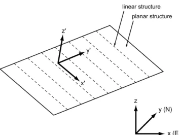
Figure 1 shows the spatial relationship between the global or geographical coordinate axes (x, y, z) and the local coor- dinate or material symmetry axes (x', y', z') for true aniso- tropic geologic structures. The geographical coordinate axes (x, y, z) are defined here as follows (Figure 1). The x axis is horizontal to the east, the y axis is horizontal to the north forming the xy plane parallel to the horizon, and the z axis is vertical to the zenith. The material symmetry axes (x', y', z') for true anisotropic (orthotropic) geologic struc- tures are then defined here as follows (Figure 1). The x' axis is aligned with linear structures (e.g., mineral elongation,

∇⋅[–K_rKsat⋅∇ h h( + e)] ndS_w

--- nSdh + wβwγw

⎝ ⎠

⎛ ⎞∂h

---∂t +

S_wαij∂εij

---∂ t

+ =q_w

∇ ∇

∂

∂xj

--- D[( _ijklεkl)^e–(S_wαijγwh)^e]+[nS_wρw+(1 n– )ρs]^eg_i= 0

striation, joint intersection), the y' axis is 90° counter-clock- wise (i.e., +π/2) from the x' axis forming the x'y' plane par- allel to planar structures (e.g. bedding, foliation, joint), and the z' axis is vertically upward from the x'y' plane (i.e., pole to planar structures). Figure 2 represents a jointed rock mass composed of an intact rock matrix with bedding planes, indi- vidual joints, and joint sets, which are true anisotropic.

3. HYDRAULIC CONDUCTIVITY TENSORS

In this section, global hydraulic conductivity tensors in equation (1) for variably saturated true anisotropic intact rock matrices, joints, joint sets, and jointed rock masses are

derived from local hydraulic conductivity tensors using coordinate transformation on the basis of the generalized Darcy’s law (Kozeny, 1927; Carman, 1937; Carman, 1938;

Carman, 1956; Parsons, 1966; Snow, 1968; Snow, 1969;

Bear, 1972). Porosities in equations (1) and (2) for variably saturated true anisotropic intact rock matrices, joints, joint sets, and jointed rock masses are also derived.

3.1. Intact Rock Matrices

The Darcy velocity for a true anisotropic intact rock matrix in the global coordinates (x, y, z), i.e., in equation (1) can be expressed as follows:

(3) where the subscript m denotes the intact rock matrix, the superscript T denotes the matrix transpose, the superscript L denotes the local tensor in the local coordinates (x', y', z') (i.e., principal axes or directions), and the other terms cor- respond to their counterparts in equation (1). Here Am is the coordinate transformation matrix for the global and local effective hydraulic conductivity tensors of the intact rock matrix (see Appendix A). In addition, the local saturated hydraulic conductivity tensor K_m^L_sat of the intact rock matrix is defined as follows (KmL

sat ij = KmL

sat ji) (Kozeny, 1927; Car- man, 1937; Carman, 1938; Carman, 1956):

K_m^L_sat=

(4) where μw is the dynamic viscosity of water, km satL is the local saturated intrinsic permeability tensor of the intact rock matrix (kmL

sat ij = kmL

sat ji), fm n= nm3/(1−nm)² is the porosity factor of the intact rock matrix, f_{m s i}= 1/180 is the shape fac- tor of the intact rock matrix in the i direction, and d_{m i} is the mean or effective diameter of the solid grains, which con- stitute the intact rock matrix, in the i direction. Here the solid grains are assumed to be ellipsoidal.

The global effective hydraulic conductivity tensor Km of the intact rock matrix can thus be calculated from its local effective hydraulic conductivity tensor KmL using the coor- dinate transformation matrix Am as follows:

(5) On the other hand, the porosity n_m of the intact rock matrix in equations (1) and (2) can be expressed as follows (Kim and Parizek, 1999b):

qm=− Km⋅∇ h( m+h_e) =–K_{m r}Km sat⋅∇ h( m+h_e)

=− AmT

K_{m r}Km satL Am⋅∇ h( m+h_e) =–AmTKmLAm⋅∇ h( m+h_e)

ρwg μw

---km satL ρwg μw

---fm n

f_{m s x′}d_{m x′}² 0 0

0 f_{m s y′}d_{m y′}² 0

0 0 f_{m s z′}d_{m z′}²

=

Km K_{m r}Km sat AmT

K_{m r}Km satL Am AmTKmLAm

= = =

Fig. 1. Spatial relationship between the global or geographical coordinate axes (x, y, z) and the local coordinate or material sym- metry axes (x', y', z') for true anisotropic geologic structures.

Fig. 2. Representation of a jointed rock mass composed of an intact rock matrix with bedding planes, individual joints, and joint sets, which are true anisotropic.

(6)

where n_m^ois the initial porosity of the intact rock matrix prior to deformation, and εm v= εm xx+εm yy+εm zz is the volumetric strain or volume dilation in the intact rock matrix.

3.2. Joints

The Darcy velocity for a true anisotropic joint in the glo- bal coordinates (x, y, z), i.e., in equation (1) can be expressed as follows:

(7) where the subscript jt denotes the joint, and the other terms correspond to their counterparts in equations (1) and (3).

Here Ajt is the coordinate transformation matrix for the glo- bal and local effective hydraulic conductivity tensors of the joint (see Appendix A). In addition, the local saturated hydraulic conductivity tensor of the joint is defined as follows (K_jt^L_{sat ij} = K^L_{jtsat ji}) (Parsons, 1966; Snow, 1968; Snow, 1969):

K_jt^L_sat= (8)

where k_jt^L_satis the local saturated intrinsic permeability tensor of the joint (kLjt

sat ij = kjtL

sat ji), fjt n= 1 is the porosity factor of the joint, fjt s i= 1/12 is the shape factor of the joint in the i direction, and b_{jt i} is the aperture of the joint in the i direction.

Here the joint is assumed to be planar and associated with linear structures, and the aperture b_{jt i} of the joint in the i direction can be expressed as follows:

i = (9)

where is the initial aperture of the joint in the i direc- tion prior to deformation, and is the joint-normal strain in the joint, which can be obtained from equation (26) or (B3).

The global effective hydraulic conductivity tensor K_jt of the joint can thus be calculated from its local effective hydraulic conductivity tensor K_jt^Lusing the coordinate trans- formation matrix A_jt as follows:

(10) On the other hand, the porosity njt of the joint in equations (1) and (2) can be expressed as follows:

(11)

3.3. Joint Sets

The Darcy velocity for a true anisotropic joint set in the global coordinates (x, y, z), i.e., in equation (1) can be expressed using equation (7) as follows:

(12) where the subscript js denotes the joint set, and the other terms correspond to their counterparts in equations (1), (3), and (7). Here A_js is the coordinate transformation matrix for the global and local effective hydraulic conductivity tensors of the joint set (see Appendix A), and w_js is the hydraulic fraction tensor of the joint set in a jointed rock mass as fol- lows:

= (13)

where bjs i is the aperture of the joint set, which is equal to the aperture b_{jt i} of the individual joints in the joint set, in the i direction, and s_{js i} is the spacing of the joint set in the i direction. Here the aperture bjs i and the spacing sjs i of the joint set in the i direction can be expressed as follows:

(14) (15) where b_{js i}^o is the initial aperture of the joint set in the i direction prior to deformation, is the joint set-nor- mal strain in the joint set, which can be obtained from equation (31) or (B3), s_{js i}^o is the initial spacing of the joint set in the i direction prior to deformation, and is the joint set-normal strain in the jointed rock mass, which can be obtained from equation (38) or (B3). In addition, the local saturated hydraulic conductivity tensor Kjs satL of the joint set is defined as follows ( ) (Parsons, 1966; Snow, 1968; Snow, 1969):

n_m 1 1–n_m^o 1 ε+ m v

--- –

=

qjt= K– jt⋅∇ h( jt+h_e) =–K_{jt r}Kjt sat∇ h( jt+h_e)

= A– KjtT jt rKjt satL Ajt⋅∇ h( jt+h_e)= – KAjtT jtLAjt⋅∇ h( jt+h_e)

Kjt satL

ρwg μw

---kjt satL ρwg μw

---fjt n

f_{jt s x′}b_{jt x′}² 0 0 0 f_{jt s y′}b_{jt y′}² 0

0 0 0

=

b_{jt i}(εjt ij) b= jt io (1 ε+ jt z′z′) x′ y′ z′, , b_{jt i}^o

εjt z′z′

Kjt =K_{jt r}Kjt sat=AjtTK_{jt r}Kjt satL Ajt =AjtTKjt LAjt

n_jt 1 2--- b_{jt x′}

b_{jt x′}

--- b_{jt y′}

b_{jt y′}

---

⎝ + ⎠

⎛ ⎞ 1

= =

qjs= −Kjs⋅∇ h( js+h_e)=–K_{js r}Kjs sat∇ h( js+h_e)

= −AjsT

K_{js r}Kjs satL Ajs⋅∇ h( js+h_e)= – KAjsT jsLAjs⋅∇ h( js+h_e)

= −AjtT

K_{jt r}wjsKjt satL Ajt⋅∇ h( jt+h_e)

= −AjsT

K_{js r}wjsKjt satL Ajs⋅∇ h( js+h_e)

wjs

b_{js x′}⁄s_{js x′} 0 0

0 b_{js y′}⁄s_{js y′} 0

0 0 b_{js z′}⁄s_{js z′}

=

b_{jt x′}⁄s_{js x′} 0 0

0 b_{jt y′}⁄s_{js y′} 0

0 0 b_{jt z′}⁄s_{js z′}

b_{js i}(εjs ij) b= js io (1 ε+ js z′z′) i =x′ y′ z′, , s_{js i}(εrm ij) s= js io (1 ε+ rm z′z′) i= x′ y′ z′, ,

εjs z′z′

εrm z′z′

K_{js sat ij}^L = K_{js sat ji}^L

(16)

where k_{js sat}^L is the local saturated intrinsic permeability ten- sor of the joint set ( ),

is the porosity factor of the joint set in the i direction, and is the shape factor of the joint set, which is equal to the shape factor of the individual joints in the joint set, in the i direction. Here the joints in the joint set are assumed to be parallel to each other and to be planar and associated with linear structures. It is also assumed that the hydraulic heads are in local equilibrium, i.e., .

The global effective hydraulic conductivity tensor K_js of the joint set can thus be calculated from its local effective hydraulic conductivity tensor KjsLusing the coordinate trans- formation matrix A_js as follows:

(17) On the other hand, the porosity n_js of the joint set in equa- tions (1) and (2) can be expressed as follows:

(18)

3.4. Jointed Rock Masses

The Darcy velocity for a true anisotropic jointed rock mass consisting of an intact rock matrix and joint sets in the global coordinates (x, y, z), i.e., in equation (1) can be expressed using equations (3) and (12) from the fact that the total water flux through the jointed rock mass is equal to the sum of individual water fluxes through the intact rock matrix and joint sets under the local hydraulic head equi- librium assumption (i.e., ) as follows:

q_rm=− qrm=− qrm=− q_rm=−

=

=

(19) where the subscript rm denotes the jointed rock mass, nn is the number of joint sets in the jointed rock mass, and the other terms correspond to their counterparts in equations (1), (3), (7), and (12). Here A_rm is the coordinate transformation matrix for the global and local effective hydraulic conduc- tivity tensors of the jointed rock mass (see Appendix A).

The global effective hydraulic conductivity tensor K_rm of the jointed rock mass consisting of an intact rock matrix and joint sets can thus be calculated from the local effective hydraulic conductivity tensors K_m^L of the intact rock matrix and K_js^Lof the joint sets using their coordinate transforma- tion matrices Am and Ajs as follows:

=

= (20)

On the other hand, the porosity n_rm of the jointed rock mass consisting of an intact rock matrix and joint sets in equations (1) and (2) can be expressed as follows:

(21)

where njst is the porosity of nn joint sets, and it is assumed that joint intersection is negligible compared with the sum of porosities of nn joint sets. Note that the porosity n_m of the intact rock matrix can be expressed by equation (6), while the porosity n_js of each joint set can be expressed by equa- tion (18).

4. MECHANICAL STIFFNESS TENSORS

In this section, global mechanical stiffness tensors in equations (1) and (2) for variably saturated true anisotropic intact rock matrices, joints, joint sets, and jointed rock masses are derived from local and global mechanical com- pliance tensors using coordinate transformation on the basis of the generalized Hooke’s law (Love, 1944; Lekhnitskii, 1963; Goodman et al., 1968; Goodman and Dubois, 1972).

Kjs satL ρwg μw

---kjs satL wjsKjt satL ρwg μw

---wjskjt satL

= = =

ρwg μw

---

f_{jt s x′}b_{jt x′}³ ⁄s_{js x′} 0 0 0 f_{jt s y′}b_{jt y′}³ ⁄s_{js y′} 0

0 0 0

=

ρwg μw

---

f_{js n x′}f_{js s x′}b_{js x′}² 0 0 0 f_{js n y′}f_{js s y′}b_{js y′}² 0

0 0 0

=

k_{js sat ij}^L =k_{js sat ji}^L f_{js n i}=b_{js i}⁄s_{js i} =w_{js ii} f_{js s i} =1 12⁄

f_{jt s i} =1 12⁄

h_js =h_jt

Kjs K_{js r}Kjs sat AjsT

K_{js r}Kjs satL Ajs AjsTKjs LAjs

= = =

n_js 1

2--- w( js x′x′+w_{js y′y′}) 1 2--- b_{js x′}

s_{js x′}

--- b_{js y′}

s_{js y′}

---

⎝ + ⎠

⎛ ⎞

= =

h_rm =h_m =h_js =h_jt Krm⋅∇ h( rm+h_e)= –K_{rm r}Krm sat⋅∇ h( rm+h_e) ArmT

K_{rm r}Krm satL Arm⋅∇ h( rm+h_e) ArmT KrmL Arm⋅∇ h( rm+h_e)= 1 n_js

js 1=

∑

nn

⎝ – ⎠

⎛ ⎞qm qjs

js 1=

∑

nn

+

1 n_js

js 1=

∑

nn

⎝ – ⎠

⎛ ⎞K_{m r}Km sat⋅∇ h( m+h_e)

K_{js r}

js 1=

∑

nn

– Kjs sat⋅∇ h( js+h_e)

1 n_js

js 1=

∑

nn

⎝ – ⎠

⎛ ⎞AmTK_{m r}Km satL Am AjsTK_{js r}Kjs satL Ajs js 1=

∑

nn

+ –

∇ h( rm+h_e)

⋅

1 n_js

js 1=

∑

nn

⎝ – ⎠

⎛ ⎞AmTKmLAm AjsTKjsLAjs js 1=

∑

nn

+ ⋅∇ h( rm+h_e) –

Krm =K_{rm r}Krm sat

1 n_js

js 1=

∑

nn

⎝ – ⎠

⎛ ⎞AmT

K_{m r}Km satL Am AjsT

K_{js r}Kjs satL Ajs js 1=

∑

nn

+

1 n_js

js 1=

∑

nn

⎝ – ⎠

⎛ ⎞AmTKmLAm AjsTKjsLAjs js 1=

∑

nn

+

n_rm n_m+n_jst n_m n_js

js 1=

∑

nn

+

= =

4.1. Intact Rock Matrices

The strain tensor for a true anisotropic intact rock matrix in the local coordinates (x', y', z') can be expressed as fol- lows:

(22) where the subscript m denotes the intact rock matrix, the superscript L denotes the local tensor in the local coordinates (x', y', z') (i.e., principal axes or directions), the superscript T denotes the matrix transpose, and the other terms correspond to their counterparts in equation (2). Here B_m is the coordi- nate transformation matrix for the global and local mechan- ical stiffness tensors of the intact rock matrix (see Appendix B). In addition, the local mechanical compliance tensor of the intact rock matrix is defined as follows

( ) (Love, 1944; Lekhnitskii,

1963):

C_m^L=

(23) where DmL is the local mechanical stiffness tensor of the

intact rock matrix ( ), E_{m i} is

Young’s modulus (modulus of elasticity) of the intact rock matrix in the i direction, νm ij is Poisson’s ratio for normal strain in the j direction due to effective normal stress of the intact rock matrix in the i direction, and Gm ij is the shear modulus (modulus of rigidity) of the intact rock matrix in the ij plane.

The effective stress tensor for the intact rock matrix in the global coordinates (x, y, z), i.e., in equation (2) can also be expressed as follows:

(24)

The global mechanical stiffness tensor D_m of the intact rock matrix can thus be calculated from its local mechanical compliance tensor C_m^L using the coordinate transformation matrix Bm as follows:

(25)

4.2. Joints

The strain tensor for a true anisotropic joint in the local coordinates (x', y', z') can be expressed as follows:

(26) where the subscript jt denotes the joint, and the other terms correspond to their counterparts in equations (2) and (22).

Here B_jt is the coordinate transformation matrix for the glo- bal and local mechanical stiffness tensors of the joint (see Appendix B), In addition, the local mechanical compliance tensor of the joint is defined as follows ( = ) (Goodman et al., 1968; Goodman and Dubois, 1972):

(27)

where D_jt^Lis the local mechanical stiffness tensor of the joint ( = ), kjt i is the stiffness of the joint in the i direction (normal stiffness if i = z' and shear stiffness if ), and bjt i is the aperture of the joint in the i direction. Here the joint is assumed to be planar and asso- ciated with linear structures, and the aperture b_{jt i} of the joint in the i direction can be expressed as follows:

(28)

where is the initial aperture of the joint in the i direction prior to deformation, and is the joint-normal strain in the joint, which can be obtained from equation (26) or (B3).

The effective stress tensor for the joint in the global coor- dinates (x, y, z), i.e., in equation (2) can also be expressed as follows:

(29) The global mechanical stiffness tensor D_jt of the joint can thus be calculated from its local mechanical compliance tensor C_jt^Lusing the coordinate transformation matrix B_jt as follows:

(30) 4.3. Joint Sets

The strain tensor for a true anisotropic joint set in the εm

{ }^L =CmL{ }σm′ ^L =BmCmBmT{ }σm′ ^L

CmL = DmL^–1

C_{m ijkl}^L =C_{m jikl}^L =C_{m ijlk}^L =C_{m klij}^L

1⁄Em x′ –νm x′y′⁄Em x′–νm x′z′⁄Em x′ 0 0 0 νm x′y′

– ⁄Em x′ 1⁄Em y′ –νm y′z′⁄Em y′ 0 0 0 νm x′z′

– ⁄Em x′–νm y′z′⁄Em y′ 1⁄Em z′ 0 0 0

0 0 0 1⁄Gm x′y′ 0 0

0 0 0 0 1⁄Gm y′z′ 0

0 0 0 0 0 1⁄Gm z′x′

D_{m ijkl}^L = D_{m jikl}^L = D_{m ijlk}^L =D_{m klij}^L

σm′

{ } D= m{ } Cεm = m–1{ } Bεm = mTDmLBm{ }εm

BmTCmL^–1Bm{ }εm

=

Dm = Cm–1=BmTDmLBm = BmTCmL^–1Bm

εjt

{ }^L =CjtL{ }σjt′ ^L= BjtCjtBjtT{ }σjt′ ^L

CjtL =DjtL^–1 C_{jt ijkl}^L

C_{jt jikl}^L = C_{jt ijlk}^L = C_{jt klij}^L

CjtL=

0 0 0 0 0 0

0 0 0 0 0 0

0 0 1 k⁄ jt z′b_{jt z′} 0 0 0

0 0 0 0 0 0

0 0 0 0 1 k⁄ jt y′b_{jt y′} 0 0 0 0 0 0 1 k⁄ jt x′b_{jt x′}

D_{jt ijkl}^L D_{jt jikl}^L =D_{jt ijlk}^L =D_{jt klij}^L i z≠ ′

b_{jt i}(εjt ij) b= jt io (1 ε+ jt z′z′) i =x′ y′ z′, , b_{jt i}^o

εjt z′z′

σjt′

{ }=Djt{ }=Cεjt jt–1{ }=Bεjt jtTDjtLBjt{ }= Bεjt jtTCjtL^–1Bjt{ }εjt

Djt =Cjt–1=BjtTDjtLBjt =BjtTCjtL^–1Bjt

local coordinates (x', y', z') can be expressed using equation (26) as follows:

(31)

where the subscript js denotes the joint set, and the other terms correspond to their counterparts in equations (2), (22), and (26). Here B_js is the coordinate transformation matrix for the global and local mechanical stiffness tensors of the joint set (see Appendix B), and r_js is the mechanical fraction ten- sor of the joint set in a jointed rock mass as follows:

r_js=

rjs= (32)

where bjs i is the aperture of the joint set, which is equal to the aperture b_{jt i} of the individual joints in the joint set, in the i direction, and s_{js i} is the spacing of the joint set in the i direction. Here the aperture bjs i and the spacing sjs i of the joint set in the i direction can be expressed as follows:

(33) (34)

where is the initial aperture of the joint set in the i direction prior to deformation, is the joint set-nor- mal strain in the joint set, which can be obtained from equation (31) or (B3), is the initial spacing of the joint set in the i direction prior to deformation, and is the joint set-normal strain in the jointed rock mass, which can be obtained from equation (38) or (B3). In addition, the local mechanical compliance tensor CjsL= DjsL−1 of the joint set is defined as follows (

= ) (Goodman et al., 1968; Good-

man and Dubois, 1972):

= (35)

where D_js^Lis the local mechanical stiffness tensor of the joint set ( = ), kjs i is the stiffness of the joint set, which is equal to the stiffness k_{jt i} of the indi- vidual joints in the joint set, in the i direction (normal stiff- ness if and shear stiffness if ), and sjs i is the spacing of the joint set in the i direction. Here the joints in the joint set are assumed to be parallel to each other and to be planar and associated with linear structures. It is also assumed that the effective stresses are in local equilibrium, i.e., .

The effective stress tensor for the joint set in the global coordinates (x, y, z), i.e., in equation (2) can also be expressed as follows:

(36) The global mechanical stiffness tensor D_js of the joint set can thus be calculated from its local mechanical compliance tensor C_js^L using the coordinate transformation matrix B_js as follows:

(37) 4.4. Jointed Rock Masses

The strain tensor for a true anisotropic jointed rock mass consisting of an intact rock matrix and joint sets in the global coordinates (x, y, z), i.e., in equation (2) can be expressed using and inverting equations (24) and (36) from the fact that the total deformation (strain) within the jointed rock mass is equal to the sum of the individual deformations (strains) within the intact rock matrix and joint sets under the local effective stress equilibrium assumption (i.e.,

) as follows:

(38)

εjs

{ }^L =CjsL{ }σjs′ ^L =BjsCjsBjsT{ }σjs′ ^L

rjs{ }εjt ^L

= =rjsCjtL{ }σjt′ ^L= rjsBjtCjtBjtT{ }σjt′ ^L

rjsBjsCjtBjsT{ }σjs′ ^L

=

1 0 0 0 0 0

0 1 0 0 0 0

0 0 bjs z′⁄s_{js z′}0 0 0

0 0 0 1 0 0

0 0 0 0 bjs y′⁄s_{js y′} 0 0 0 0 0 0 b_{js x′}⁄s_{js x′}

1 0 0 0 0 0

0 1 0 0 0 0

0 0 bjt z′⁄s_{js z′}0 0 0

0 0 0 1 0 0

0 0 0 0 bjt y′⁄s_{js y′} 0 0 0 0 0 0 b_{jt x′}⁄s_{js x′}

b_{js i}(εjs ij) b= js io (1 ε+ js z′z′) i =x′ y′ z′, , s_{js i}(εrm ij) s= js io (1 ε+ rm z′z′) i =x′ y′ z′, ,

b_{js i}^o

εjs z′z′

s_{js i}^o

εrm z′z′

C_{js ijkl}^L C_{js jikl}^L = C_{js ijlk}^L =C_{js klij}^L

CjsL =rjsCjtL

0 0 0 0 0 0

0 0 0 0 0 0

0 0 1 k⁄ js z′s_{js z′}0 0 0

0 0 0 0 0 0

0 0 0 0 1 k⁄ js y′s_{js y′} 0 0 0 0 0 0 1 k⁄ js x′s_{js x′}

D_{js ijkl}^L D_{js jikl}^L = D_{js ijlk}^L = D_{js klij}^L

i =z′ i z≠ ′

σjs′ =σjt′

σjs′

{ }=Djs{ }=Cεjs js–1{ }=Bεjs jsTDjsLBjs{ }= Bεjs jsTCjsL^–1Bjs{ }εjs

Djs =Cjs–1=BjsTDjsLBjs= BjsTCjsL^–1Bjs

σrm′ =σm′ =σjs′ =σjt′

εrm

{ } C= rm{σrm′ } F= rmT CrmL Frm{σrm′ }

= 1 n_js

js 1=

∑

nn

⎝ – ⎠

⎛ ⎞ ε{ }m { }εjs js 1=

∑

nn

+

= 1 n_js

js 1=

∑

nn

⎝ – ⎠

⎛ ⎞FmTCmLFm{ }σm′ FjsTCjsLFjs{ }σjs′ js 1=

∑

nn

+

= 1 n_js

js 1=

∑

nn

⎝ – ⎠

⎛ ⎞FmTCmLFm FjsTCjsLFjs js 1=

∑

nn

+ {σrm′ }

where the subscript rm denotes the jointed rock mass, is the local mechanical compliance tensor of the

jointed rock mass ( = ), nn is

the number of joint sets in the jointed rock mass, and the other terms correspond to their counterparts in equations (2), (24), (29), and (36). Here is the local mechanical stiffness tensor of the jointed rock mass ( = = = ). In addition, F_rm, F_m, and F_js are the coordinate transformation matrices for the global and local mechanical compliance tensors of the jointed rock mass, intact rock matrix, and joint set, respectively (see Appendix C), and n_js is the porosity of each joint set as follows:

(39) The global mechanical compliance tensor C_rm of the jointed rock mass consisting of an intact rock matrix and joint sets can thus be calculated from the local mechanical compliance tensors C_m^L of the intact rock matrix and C_js^Lof the joint sets using their coordinate transformation matrices F_m and F_js as follows:

(40) The effective stress tensor for the jointed rock mass con- sisting of an intact rock matrix and joint sets in the global coordinates (x, y, z), i.e., in equation (2) can also be expressed as follows:

(41) where B_rm is the coordinate transformation matrix for the global and local mechanical stiffness tensors of the jointed rock mass (see Appendix B).

The global mechanical stiffness tensor D_rm of the jointed rock mass consisting of an intact rock matrix and joint sets can thus be calculated from its global mechanical compli- ance tensor C_rm by inverting as follows:

(42)

5. CONCLUSIONS

A series of global hydraulic conductivity and mechanical stiffness tensors for variably saturated true anisotropic intact rock matrices, joints, joint sets, and jointed rock masses was formulated to expand the fully coupled poroelastic govern- ing equations presented by Kim (2004) for groundwater flow and solid skeleton deformation in porous geologic media to those for fractured and fractured porous geologic media. The global hydraulic conductivity tensors were derived

from the local hydraulic conductivity tensors using coordi- nate transformation on the basis of the generalized Darcy’s law. The global mechanical stiffness tensors were then derived from the local or global mechanical compliance tensors using coordinate transformation on the basis of the gener- alized Hooke’s law. Although the global hydraulic conduc- tivity and mechanical stiffness tensors formulated in this paper will not apply to all types of geologic media, they can find some useful applications in many problems associated with fully coupled groundwater flow and solid skeleton deformation in geologic media.

APPENDIX A: COORDINATE TRANSFORMATION TENSOR FOR HYDRAULIC CONDUCTIVITY TENSORS

In equations (3), (7), (12), and (19), Am, Ajt, Ajs, and Arm

are the coordinate transformation matrices for the global and local effective hydraulic conductivity tensors of an intact rock matrix (m), joint ( jt), joint set ( js), and jointed rock mass (rm), respectively, as follows (Clebsch, 1994;

Kim, 2003):

I = m, jt, js, rm (A1)

where the nine components are the direction cosines between the local coordinates (x', y', z') (i.e., principal axes or direc- tions) and the global coordinates (x, y, z), and thus they can be determined from geologic angle measurements of planar (x', y') structures (e.g., bedding, foliation, joint) and linear (x') structures (e.g., mineral elongation, striation, joint inter- section) using the mathematical equations suggested by Kim (2005b). Here l, m, and n stand for x, y, and z, respectively.

Note that .

APPENDIX B: COORDINATE TRANSFORMATION TENSOR FOR MECHANICAL STIFFNESS TENSORS

In equations (22), (26), (31), and (41), B_m, B_jt, B_js, and B_rm are the coordinate transformation matrices for the global and local mechanical stiffness tensors of an intact rock matrix (m), joint ( jt), joint set ( js), and jointed rock mass (rm), respectively, as follows (Cook et al., 1989; Kim, 2003):

I = m, jt, js, rm (B1)

CrmL = DrmL^–1

C_{rm ijkl}^L C_{rm jikl}^L =C_{rm ijlk}^L = C_{rm klij}^L

DrmL

D_{rm ijkl}^L D_{rm jikl}^L D_{rm ijlk}^L D_{rm klij}^L

n_js 1

2--- w( js x′x′+w_{js y′y′}) 1 2--- b_{js x′}

s_{js x′}

--- b_{js y′}

s_{js y′}

---

⎝ + ⎠

⎛ ⎞

= =

Crm FrmT CrmL Frm 1 n_js

js 1=

∑

nn

⎝ – ⎠

⎛ ⎞FmTCmLFm FjsTCjsLFjs js 1=

∑

nn

+

= =

σrm′

{ }=Drm{ }=Bεrm rmT DrmL Brm{ }= Bεrm rmT CrmL^–1Brm{ }εrm

Crm–1{ }εrm

=

Drm = BrmT DrmL Brm=BrmT CrmL^–1Brm = Crm–1

AI

l_x′m_x′n_x′

l_y′m_y′n_y′

l_z′m_z′n_{n′ I}

=

Ajs =Ajt

B_I

lx2′ mx2′ nx2′ lx′mx′ mx′nx′ nx′lx′

l_y2′ m_y2′ n_y2′ l_y′m_y′ m_y′n_y′ n_y′l_y′

l_z2′ m_z2′ n_z2′ l_z′m_z′ m_z′n_z′ n_z′l_z′

2l_x′l_y′2m_x′m_y′2n_x′n_y′l_x′m_y′+l_y′m_x′m_x′n_y′+m_y′n_x′n_x′l_y′+n_y′l_x′

2ly′lz′2my′mz′ 2ny′nz′ly′mz′+lz′my′ my′nz′+mz′ny′ ny′lz′+nz′ly′

2l_z′l_x′2m_z′m_x′ 2n_z′n_x′l_z′m_x′+l_x′m_z′ m_z′n_x′+m_x′n_z′ n_z′l_x′+n_x′l_z′

=

I