IEG 환경지질연구정보센터

전체 글

(1)Geosciences Journal Vol. 11, No. 4, p. 369 − 376, December 2007. Estimating polar marine free-air gravity anomalies from dense radar altimeter data Jeong Woo Kim*,† Department of Geoinformation Engineering, Sejong University, Seoul 143-747, Korea Bang Yong Lee Korea Polar Research Institute, Korea Ocean Research and Development Institute, Incheon 406-840, Korea. ABSTRACT: Geological free-air gravity anomalies of the polar marine areas were estimated from dense ERS1 radar altimeter data. Data processing techniques were developed to deal with data gaps from the seasonal ice coverage, directional variations of the ascending and descending orbital data tracks, and other high-latitude mapping problems. To reduce along-track data distortions, the ERS1 168 altimetry data were geodetically co-phased and spectral correlation filtered. Geoid undulations were first estimated and converted to the free-air gravity anomalies by Brun’s formula and the fundamental equation of geodesy. The results in the open waters of the Barents and Kara Seas of the Russian Arctic show good coherence with global model and shipborne data, whereas along the coastline, strong ocean currents, possible tidal model inaccuracies, and poor data coverage limit the coherence. The approach uses local satellite altimetry to update reference gravity models in the polar regions. It thus has considerable utility for resolving details of the polar marine gravity field as global warming removes the ice cover and the cross-track distance of altimeter missions decreases. Key words: free-air gravity anomaly, ERS1 altimeter data, geoid undulation, Barents and Kara Seas. 1. INTRODUCTION Satellite radar altimeter observations have been increasingly used to determine free-air gravity anomalies for geological studies of the remote marine regions of the Earth (Hofmann-Wellenhof and Moritz, 2006, Seeber, 2003). Altimetry satellite missions are typically near polar orbiting and thus provide especially dense spatial coverage over the polar regions where the orbital tracks converge. To take advantage of the enhanced coverage in the polar regions, this study developed procedures to reduce the non-geological noise in the altimetry-derived free-air gravity estimates. Specifically, the radar altimeter data from the first European Remote Sensing Satellite (ERS1) were used to predict the free-air gravity anomalies (FAGA) of the Barents and Kara Seas in the Russian Arctic between the area 20o–70o E and 68o–78o N. The orbital inclination of this mission was roughly 98.5o. The effect of this near polar orbit limited the satellite’s track coverage to between 81.5o *Corresponding author: [email protected] † Also at: Department of Geomatics Engineering, University of Calgary, AB, T2N 1N4, Canada. North and South latitudes. ERS1 was operated to produce repeat orbits at 3-, 5-, and 168-day intervals. The 3- and 35-day mission data can be stacked to reduce noise, but the spacing between tracks is appropriate only for the most regional geological applications. The 168-day mission was run twice so that the ground tracks of the second mission were in between those of the first. Thus, no overlapping tracks were obtained, but the effective track spacing provided relatively dense spatial coverage. For example, the two 168-day mission data obtained track spacing of about 8 km at the equator and about 2.3 km for the study area (73o N). Hence, this study considered only the 168-day mission data for recovering geologically useful gravity anomalies. To derive FAGA from satellite radar altimetry, vertical deflections of the geoidal undulations are often used (Sandwell, 1990, 1992). This approach minimizes the need for orbital and cross-over adjustments, because the gradient solutions are used. However, the approach includes track-line noise in its predictions and regional distortions that may be important in studying the gravity effects of large-scale crustal features. An alternative method derives free-air gravity anomalies directly from geoid undulations using the fundamental equation of geodesy and Brun’s formula (Heiskanen and Moritz, 1967). This method incorporates orbital cross-over adjustments and spectral correlation filtering of neighboring orbital data tracks, as well as maps from the ascending and descending data sets to estimate geoid undulations with maximum signal-to-noise ratios (von Frese et al., 1997). This approach enhances the recovery of gravity at all wavelengths, because it is based on determining geoid undulations as accurately as possible. Furthermore, this approach permits procedures to be implemented in the wavenumber domain that are effective for attenuating track-line noise (Kim et al., 1998), especially at high latitudes where ascending and descending orbits cross each other at relatively high angles. This study presents a direct method to recover free-air gravity anomalies of the Barents and Kara Seas between 20o–70o E and 68o–78o N from the 168-day mission of the ERS1. This application calculates gravity anomalies from dense polar altimeter data that includes gaps from ice cov-.

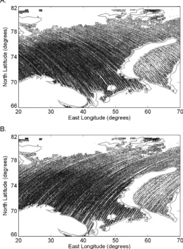
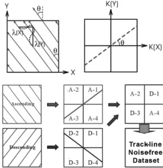
(2) 370. Jeong Woo Kim and Bang Yong Lee. erage and considerable track-line noise. For quality assessment, the estimated FAGA are compared against the KMS02 global gravity model (Andersen et al., 2003) and shipborne gravity obtained by the Lamont-Doherty Earth Observatory of Columbia University (NGDC, 1998). 2. THEORETICAL BACKGROUND 2.1. Estimating Free-air Gravity Anomalies from Geoid Undulations From the geometry of satellite radar altimetry shown in Figure 1 (e.g., von Frese et al., 1999, Kim, 1996), we can estimate the sea surface height, SSH, by SSH = Hs − Ha. (1). Here, the sea surface height, SSH, is the distance between the footprint of the radar signal on the sea surface and the reference ellipsoid, where Hs is the altitude of the ERS1 satellite from the reference ellipsoid, and Ha is the distance from the footprint on the sea surface to the ERS1 satellite. The only observable of satellite radar altimetry, Ha, can be calculated by measuring the two-way travel time of an electromagnetic pulse from the onboard radar transmitter and antenna system. The radar pulse passes through a distance of about 1,560 km for ERS1 (i.e., 2×780 km) in the atmosphere that is not an ideal vacuum and contains materials causing time delays. Thus, corrections for dry and wet tropospheric as well as ionospheric effects are made in addition to the instrumental error corrections (Kim, 1996). In general, SSH is obscured by many factors and must be corrected for the time-varying effects of the Earth’s tidal response by the Moon and the Sun. In this study, dynamic ocean tidal corrections were implemented using the CSR3.0. Fig. 1. Geometry of satellite radar altimetry. The observed altimeter height can be obtained by removing the sea surface height from the orbital height. The free-air gravity anomaly can be calculated from the geoid undulation that was estimated from the mean sea surface height.. and FES95.2.1 models (CLS, 1993). The corrected sea surface height, SSHc, is given by SSHc = GU + DSST + e. (2). where GU is geoid undulation, DSST is the dynamic sea surface topography, and e is the error due to instrumental and other uncertainties. We used the OSU91 DSST global model (Rapp et al., 1991) to account for DSST contributions and spectral correlation filtering of the related N estimates to reduce the errors, e. The free-air gravity anomaly, Δg in Gal, can be obtained from the geoid undulation, GU in cm, because Brun’s formula (Heiskanen and Moritz, 1967) relates them to the disturbing potential, T, in Gal×cm by as follows GU = T/γ. (3). where γ is normal gravity in Gal. The disturbing potential T represents the gravitational potential of the mass that deviates from the standard homogeneous ellipsoidal Earth so that inhomogeneities in the Earth are represented by proportional changes in the GU. The fundamental equation of geodesy (Heiskanen and Moritz, 1967) also relates the gravity anom-. Fig. 2. Fig. 2. ERS1 168-day mission data coverage of the Barents and Kara Seas includes 115309 ascending track points (panel A) and 116163 descending track points (panel B)..

(3) Polar marine free-air anomalies from radar altimetry. alies, Δg, and the disturbing potential, T, as Δg = ( –∂T ⁄ ∂r ) – 2T ⁄ R. (4). where R is the Earth’s radius in cm and the radial (r) gradient of the gravity disturbance T(=GU·γ) can be calculated from a spectral filter (von Frese et al., 1999). 2.2. Wavenumber Correlation Filtering Gravity measurements at repeat stations or stations that are close to each other compared to depth of the sea floor map highly correlated geological components. Furthermore, enhancing the anomaly correlations in these observations improves the geological signal(S)-to-noise(N) ratio 1 as N/S = 1 ---------- – 1, where CC is the correlation coefficient CC (Foster and Guinzy, 1967, Kim, 1996). Wavenumber correlation filtering can improve the feature correlations in adjacent tracks and between co-registered maps made from the ascending and descending modes of satellite observations. This improvement can greatly enhance the estimation of the geological components in the altimetry-derived gravity anomalies (Kim, 1996, von Frese et al., 1997). Correlative anomaly features between co-registered data sets can be extracted by using the wavenumber correlation spectrum (von Frese et al., 1997) given by Xk ⋅ Yk CCk = cos ( Δθ k ) = --------------Xk Yk where the k-th wavevectors Xk = Xk e. –jθX. k. and Yk = Yk e. (5). – jθY. k. 371. tion. In this study, one- and two-dimensional wavenumber correlation filters were applied to extract common components between adjacent ERS1 data tracks and the co-registered geoid undulation maps derived from the ascending and descending orbital data observations. 2.3. Track-line Noise Attenuation In satellite, airborne, and shipborne geophysical surveys, data are commonly collected along nearly parallel lines where the observation interval is relatively short compared to the distance between the lines. Maps from these line data are more strongly aliased and distorted across-track than along-track. This distortion appears as a washboard effect or track-line noise parallel to the survey lines. Survey line data also tend to be reduced and processed alongtrack, so that processing errors can readily enhance trackline noise. To reduce this systematic noise, spectral differences resulting from the different survey azimuths can be exploited (Kim et al., 1998). This approach is simplified in Figure 3, where the upper left panel shows the noise and line directions that both subtend an angle of θ counterclockwise from the reference direction or the Y-axis. The λ(X) and λ(Y) wavelength components of track-line noise in the X-and Y-directions, respectively, are related by tan θ = λ(X)/λ(X). The spectral components of the noise occur in the quadrants which are orthogonal to the direction of the lines, because the wavenumber, k, and wavelength, λk, are inversely related by k = 2π/λk, so that. (6). have respective amplitudes Xk and Yk , and phase angles θ Xk and θ Yk with the phase difference Δθk = (θ Yk – θ Xk ) , and j = –1. The correlation coefficient CCk between the k-th wavenumber components Xk and Yk is simply the cosine of the shift or difference in the component phases. One- and two-dimensional wavenumber correlation filtering has been used to extract static lithospheric components of the satellite magnetometer observations (Alsdorf et al., 1994, Kim, 1996) and to isolate the crustal isostatic component in gravity observations (e.g. Leftwich et al., 2005). The procedure amounts to using the correlation spectrum to design notch filters that pass only the wavenumber components Xk and Yk which correlate at the desired coefficient levels. Inversely transforming these components yields the data domain representations of the correlated features. As with any spectral filtering application, the filtered output must be compared against the input signals to judge the reasonableness of the results and to establish the most effective values of the CCk to use in any investiga-. Fig. 3. Track-line geometries in the spatial (upper left panel) and corresponding amplitude spectrum (upper right panel) domains. Trackline noise can be suppressed from the spectrum reconstruction of quadrants A-2, A-4, D-1, and D-3 as shown in the lower right panels..

(4) 372. λ(X ) k(Y ) tanθ = ------------ = ----------λ(Y ) k(X ). Jeong Woo Kim and Bang Yong Lee. (7). Accordingly, spectral distortions due to track-line noise predominate in the pair of symmetric quadrants shown in the upper right panel of Figure 3, whereas the noise is minimum in complementary pair of symmetric quadrants. The predominant track-line noise effects in the ascending and descending data sets are in mutually exclusive spectral quadrants. Thus, we can reconstruct the spectrum from the four cleaner quadrants to produce a map of the data with substantially reduced track-line noise (Kim et al., 1998). The map obtained by inversely transforming the reconstructed spectrum can be compared to the ascending and descending data maps to assess the performance of this approach for suppressing track-line noise (Figure 3). 3. DATA PROCESSING To estimate residual geoid undulations from the satellite altimeter tracks, we used the remove-and-restore technique (Bašic´ and Rapp, 1992) using the OSU91A gravity model (Rapp et al., 1991) as the reference gravity field that was removed to residualize the observed signals. The residual geoid undulations were then processed for residual free-air gravity anomalies to which the reference gravity anomalies were restored to predict the total free-air anomalies. The sections below describe additional details of the data processing. 3.1. Pre-processing The ERS1 168-day OPR02 data resolution for the study area is about 2.3 km between tracks at 73o N and 7 km along track. The radar altimeter is a nadir looking instrument with a footprint of a few kilometers depending on the surface slope. The 7-km along track spacing is the effective altimeter footprint dictating the observable wavelengths which are roughly two times the footprint and greater. However, newer altimeter missions like ICESat (Zwally et al., 2002) with its footprint that is two orders of magnitude smaller than the ERS1 footprint offer the promise of resolving even smaller details of the marine gravity field. In processing the one-second ERS1 observations, appropriate correction terms determined from various models provided with the data were applied. These correction terms were also used to assess the quality of the data, where for example extreme values in significant wave height or dry and wet tropospheric corrections marked unreliable observations. The screened tracks were then grouped into ascending and descending data sets based on their local times for performing one-dimensional wavenumber correlation filtering (von Frese et al., 1997). Figure 2 gives the 115,309 ascending (Panel A) and 116,163 descending (Panel B) ERS1 observations that were extracted for this study.. Reference geoid undulations values were derived from the OSU91A spherical harmonic gravity model to degree and order of 360 (Rapp et al., 1991) and removed from observed values. Static components of the sea surface topography determined from the degree and order 10 coefficients of the OSU91A model (Kim and Rapp, 1990) were also removed. 3.2. Track Analysis The tracks surviving the pre-processing were then analyzed for coherent signals that include the crustal components. The data were separated into groups of ascending and descending tracks. The data interval along the track is one second or about 7 km. However, altimeter errors, landand ice-masses, etc. produce gaps in the coverage. Therefore, tracks were eliminated with 60% or that are shorter than 20 km and thus offered only a few points for analysis. For correlation filtering, the tracks were sorted next into nearest neighbor pairs. A co-phasing procedure (Kim, 1996) was used to resample the data for each track pair at a 7-km interval so that the resampled data points were aligned exactly opposite to each other across the two tracks. The co-phased tracks were then correlation filtered for the wavenumber components with CCk >0.8. Stacking or averaging the inverse transformations of these components estimated the static signals with enhanced crustal effects between the tracks. After spectral correlation filtering, the mean correlation coefficient between neighboring track pairs improved from 0.76 to 0.92. The study area is sufficiently extensive (>1,000×1,000 km) that least-squares cross-over adjustments must be applied to the correlation filtered tracks to reduce regional variations in the data from satellite orbit errors (e.g. Rapp, 1985). In the Geosat GM data of the southern oceans, for example, Kim (1996) observed cross-over differences up to 100 cm that were reduced to 10 cm level after the cross-over adjustment. The cross-over adjustment was performed using the intersections of the ascending and descending tracks across the study region (Knudsen, 1987). With this procedure, constant biases in the tracks related mostly to the regional orbital errors were removed. The data were processed next into maps for further correlation filtering to suppress additional noise components. 3.3. Map Analysis The processed ascending and descending data sets of residual geoid undulation estimates were gridded using a tensioned cubic spline. The grid spacing for the ascending and descending maps was 15 minutes in longitude and 5 minutes in latitude in general conformance with the original data spacing. To make the analysis more manageable, the two data sets were further sub-divided into eastern.

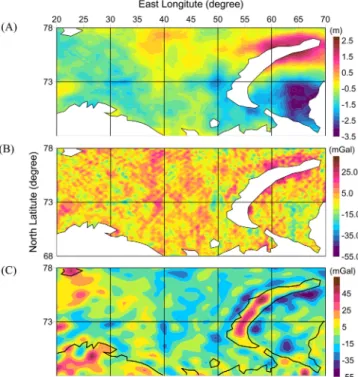
(5) Polar marine free-air anomalies from radar altimetry. (20o–55oE) and western (35o–70o E) sectors. These sectors were taken with 20o overlap to help reduce edge effects in recombining the data sets. The coefficient of correlation between the eastern sector ascending and descending data maps was 0.95, whereas it was 0.86 for the western sector maps. To improve the correlations and enhance the geological components, correlation filters were applied to pass the wavenumber components in the eastern sector maps that correlated at 0.95 and higher, whereas the western sector maps were filtered for wavenumber component correlations of 0.86 and greater. The spectral correlation filtering improved the correlation between the ascending and descending maps of the eastern and western sectors by slightly more than 4% and about 11%, respectively. The sector maps were then recombined into an ascending data map and a descending data map. For each sector map, the spectral quadrants from the ascending and descending data components were reconstructed into the spectrum with greatly suppressed track-line noise. To suppress the higher frequency noise further, these results were also lowpass filtered for wavelengths roughly greater than two times the grid interval. Figure 4(A) gives the geoid undulation estimates for the Barents and Kara Seas from the ERS1 168-day mission altimeter data. The marine altimetry directly measured undulation variations that now must be converted to related gravity anomalies using Burns’ formula (Equation 3) and the. Fig. 4. (A) Geoid undulations of the Barents and Kara Seas from ERS1 168-day mission altimetry estimates. (B) Residual free-air gravity anomalies from the geoid undulations in (A) relative to the reference OSU91A free-air gravity anomalies in (C).. 373. fundamental equation of geodesy (Equation 4). The spherical coordinate data in Figure 4(A) were resampled into a Cartesian grid (Kim and Lee, 2002) using the Lambert Conformal Conic Projection (Synder, 1987) to apply the fast Fourier transform vertical derivative filter coefficients for estimating gravity anomalies according to Equation 2. Figure 4(B) shows the resulting residual freeair gravity anomaly estimates projected back into spherical coordinates. To obtain the total free-air gravity anomalies, the reference free-air anomalies from OSU91A in Figure 4(C) were added back to the residual gravity anomalies in Figure 4(B). Figure 5(A) gives the total free-air gravity anomaly estimates derived from the ERS1 168-day satellite radar altimeter data for the study region. 4. QUALITY ASSESSMENT To investigate the veracity of the ERS1 altimetry-implied FAGA, comparisons were made with the KMS02 global gravity model (Andersen et al., 2003) and shipborne gravity survey profiles collected for the study region by the Lamont-Doherty Earth Observatory of Columbia University (NGDC, 1998). Figure 5(B) shows the KMS02 global model estimates that incorporated gravity data from the Geosat GM and ERS1, as well as ERM60-63 of ERS2 mis-. Fig. 5. (A) Total (residual in Fig. 4.B + reference in Fig. 4.C) freeair gravity anomaly estimates. (B) Free-air gravity anomaly from the KMS02 model. Red profiles delineate shipborne survey lines #1 and #2. (C) Differenced free-air gravity anomalies (B–A) of the study area..

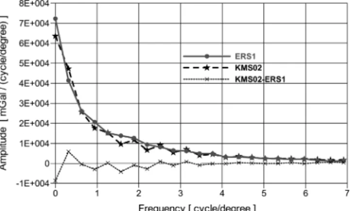
(6) 374. Jeong Woo Kim and Bang Yong Lee. Table 1. Statistical comparison of free-air gravity anomaly estimates in mGal between ERS1 168-day mission data and the global model predictions of KMS02. Gravity Model ERS1 KMS02. (Min, Max). Mean. (-66.6, 70.1) (-77.0, 129.1). -5.5 -5.4. Standard Deviation 16.2 16.3. Correlation Coefficient 0.779. sions. This model used Topex/Poseidon and ERS2 exact repeat mission data to obtain significantly improved intermediate wavelength (100–250 km) components of the gravity field (Andersen et al., 2003). This model shows good similarity to ship data where around Iceland, for example, the rms difference between the ship and KMS02 data was reported to be only 4.2 mGal (Denker et al., 2005). Table 1 compares the amplitude statistics between the two sets of gravity estimates. Overall, correlation coefficient (CC) between the ERS1 free-air anomaly estimates in this study and KMS02 model prediction is 0.779. Although the mean and the standard deviation (1σ) of the two data sets are nearly identical, the maximum values of the amplitude ranges are somewhat different. The maxima of the two data sets are found in central Novaya-Zymlaya Island where no satellite altimetry returns were observed. Figure 5(C) shows the ERS1 free-air gravity estimates subtracted from the KMS02 predictions. The major differences occur on shore and near the shorelines, such as along the coast of Novaya-Zymlaya Island. These differences as well as the differences in minimum and maximum values (Table 1) may reflect the particular improvement of the KMS02 model in the coastal region (Anderson et al., 2003), whereas the ERS1 estimates are restricted to open water altimetry observations. The differences in the southcentral Kara Sea (Fig. 5(C)) reflect the excessive pruning of the ERS1 data in this region because the tracks were either too short or gap-dominated. Figure 6 shows the radially averaged values of the amplitude spectra of the two models. The averaged amplitudes were calculated to frequency 7 at the interval of 0.05 cycle/degree. The shorter wavelength components greater than 3 cycles/degree in the two models are relatively coherent, and only slightly less coherent for the longer wavelength components. Overall, the ERSI model estimates using the OISU91 DSST and reference gravity models (Rapp et al., 1991) compare well with the more recent KMS02 model estimates (Anderson et al., 2003). Figure 7 compares the ERS1 and KMS02 anomaly estimates with two shipborne gravity profiles obtained by the Lamont-Dolherty Earth Observatory of Columbia University (NGDC, 1998) along the tracks shown in Figure 5. Lines #1 and #2 in Figure 5 were respectively measured between 2-6 Sep. and 12-14 Sep. 1973. These analog data (#v3011) were collected in September, 1973 by a Graf-. Fig. 6. Radially averaged values of the amplitude spectra of the ERS1 and KMS02 free-air gravity anomalies. The averaged amplitudes were calculated to frequency 7 at the interval of 0.05 cycle/ degree.. Fig. 7. Comparisons of the free-air anomaly estimates along shipborne survey lines #1 (A) and #2 (B) in Figure 5 obtained by the Lamont-Doherty Earth Observatory.. Askania GSS2-12 sea gravimeter with mean error of about 2.0 mGal (Valliant et al., 1976). Table 2 compares the correlation coefficients between the various anomaly estimates. For the shipborne Line #1, the ERS1 and KMS02 profiles have correlation coefficients of 0.799 and 0.988, respectively, whereas Line #2.

(7) Polar marine free-air anomalies from radar altimetry. Table 2. Comparison of correlation coefficients along the shipborne survey lines #1 (unshaded) and #2 (shaded) shown in Figure 5. Line 1 Line 2 SHIP ERS1 KMS02. SHIP. ERS1. KMS02. 0.799 0.770 0.988 0.967. 0.799 0.770 0.806 0.833. 0.988 0.967 0.806 0.833 -. correlates with coefficients of 0.770 and 0.967, respectively. The ERS1 and KMS02 estimates along Lines #1 and #2 correlate at 0.806 and 0.833, respectively. Relative to the ERS1 and KMS02 estimates, the shipborne gravity profiles are systematically 10-12 mGals higher due probably to the different reference ellipsoids used in processing of the gravity data sets. In addition, the ship lines correlate more strongly with the KMS02 than the ERS1 profiles because the ship data in the study region constrain the KMS02 coefficients, but not the OSU91A reference model which is the basis of the ERS1 predictions. Thus, exchanging the OSU91A model for the KMS02 coefficients for defining the residual geoid undulations can make the ERS1 estimates conform more closely to the ship data. In general, the accuracies of the residual geoid undulation and related free-air anomaly estimates will improve as reference gravity models for the region improve. 5. SUMMARY AND CONCLUSIONS Free-air gravity anomalies were estimated for the Barents and Kara Seas of the Russian Arctic from dense ERS1 168-day radar altimeter data. The tracks were sorted into nearest neighbor pairs and processed for residual geoid undulations using a reference gravity model. The residual undulations were then geodetically co-phased and correlation filtered to enhance geological gravity signals from sources located at depths greater than the track spacing. The tracks were also cross-over adjusted to help account for regional variations in the data from satellite orbit errors. The resultant undulations from the ascending and descending sets of tracks were gridded and spectrally filtered for directly correlative features to enhance the geological components further. To suppress track-line noise effects, the data spectrum was reconstructed from the spectra of the two maps and low-pass filtered for the final estimate of the residual geoid undulations of the study area. The undulations were projected from spherical into Cartesian coordinates and radially differentiated for residual free-air anomaly estimates, which were projected back into spherical coordinates (Fig. 4(C)) and added to the reference gravity field to estimate the total free-air gravity anomalies. 375. of the study region (Fig. 5(A)). For the Barents and Kara Seas, the results show good coherence with global model and shipborne data over open waters, whereas along the coastline, strong ocean currents, possible tidal model inaccuracies, and poor data coverage limit the coherence. Correlation of the ERS1 profile from this study with the ship lines showed weaker coherence than the KMS02 model, not only because the ship data constrain the KMS02, but also a greater amount of more recent data was incorporated in the model. By exchanging the OSU91A model for the newer coefficients can make our estimates conform more closely to the local data. However, this approach basically uses altimetry to update existing gravity model predictions over local spherical patches of open sea. It improves the coherence and thus the signal-to-noise ratio of geological signals between neighboring tracks and co-registered maps made at different local times. As opposed to global approaches, it can take maximum advantage of any enhancement in the local coverage like the great densification of orbital altimetry tracks in the polar regions. Thus, these procedures have considerable utility for mapping the higher resolution details of the polar marine gravity field as global warming removes more and more ice cover and the cross-track distance of satellite altimetry missions decreases. ACKNOWLEDGEMENTS: Elements of this study were financially supported by the National Research Lab. Project (M1-0302-00-0063) of Korea Ministry of Science & Technology and by Korea Polar Research Institute Project (COMPAC, PE07030).. REFERENCES Alsdorf, D.E., von Frese R.R.B., Arkani-Hamed, J., and Noltimier, H.C., 1994, Separation of lithospheric, external, and core components of the south polar geomagnetic field at satellite altitudes, J. Geophys. Res., 99(B3), 4655−4668. Andersen, O.B., and Knudsen, P., 1998, Global marine gravity field from the ERS-1 and Geosat geodetic mission altimetry, J. Geophys. Res., 103(C4), 8129−8138. Andersen, O.B., Knudsen, P., Kenyon, S., and Trimmer, R., 2003, KMS2002 global marine gravity field, bathymetry and mean sea surface, poster, IUGG 2003, Sapporo, Japan. Bašic´, T. and Rapp, R.H., 1992, Oceanwide prediction of gravity anomalies and sea surface heights using Geos-3, Seasat, and Geosat altimeter data and ETOPO5U bathymetric data, Dept. of Geodetic Science and Surveying Report 416, The Ohio State University, Columbus, OH. CLS., 1993, Quality Assessment of CERSAT Altimeter OPR Products, OC-NT-93.005, CDs, 43, 44, 45, 46, 49, 52, 53, 54, 55. Denker, H., Barriot, J.-P., Barzaghi, R., Forsberg, R., Ihde, J., Kenyeres, A., Marti, U., and Tziavos, I.N., 2005, Status of the European Gravity and Geoid Project EGGP, Proceedings of IAG Internat. Symp. “Gravity, Geoid and Space Missions - GGSM2004”, v.129, 125−130. Foster, M.R. and Guinzy, N.J., 1967, The coefficient of coherence: its estimation and use in geophysical data processing. Geophysics,.

(8) 376. Jeong Woo Kim and Bang Yong Lee. 32(4), 602−616. Fowler, C.M.R., 2005, The Solid Earth – An Introduction to Global Geophysics (2nd ed.), Cambridge University Press. Heiskanen, W.A. and Moritz, H., 1967, Physical Geodesy, W.H. Freeman and Company San Francisco, 364p. Hofmann-Wellenhof, B. and Moritz, H., 2006, Physical Geodesy (2nd ed.), Springer Wien NewYork, 403p. Kim, J.W., 1996, Spectral Correlation of Satellite and Airborne Geopotential Field Measurements for Lithospheric Analysis, Ph.D. Dissertation (unpubl.), Department of Geological Sciences, The Ohio State University, Columbus, Ohio, 171p. Kim, J.W., 2002, Recovery of Lithospheric Magnetic Components in the Satellite Magnetometer Observations of East Asia, Korean J. of Geophysical Exploration, 5(3), 157−168. Kim, J.W., Kim, J.H., von Frese, R.R.B., Roman, D.R., and Jezek, K.C., 1998, Spectral attenuation of track-line noise, Geophys. Res. Lett., 25(2), 187−190. Kim, J.W. and Lee, D.C., 2002, Distortions of spherical data in the wavenumber domain, Korean J. of Remote Sensing, 18(3), 171− 179. Kim, J.-H. and Rapp, R., 1990, Major datasets and fields in the area of gravimetric and altimetric research, OSU Internal Report, Department of Geodetic Sciences and Surveying, The Ohio State University, Columbus, OH. Kim, J.-H., 1996, Improved Recovery of Gravity Anomalies from Dense Altimeter Data, Report No. 437, Department of Geodetic Science and Surveying, The Ohio State University. Knudsen, P., 1987, Adjustment of satellite altimeter data from crossover differences using covariance relations for the time varying components represented by Gaussian functions, Proc. IAG Symposia TOME II, 617−628. Leftwich, T., von Frese, R.R.B., Potts, L., Kim, H.R., Roman, D.R., Taylor, P.T., and Barton, M., 2005, Crustal modeling of the North Atlantic from spectrally correlated free-air terrain gravity, J. Geodynamics, 40, 23−50. NGDC., 1998, Marine trackline geophysics data CD-ROM set, U.S. Dept. of Commerce, NOAA, National Geophysical Data Center, Boulder, Colorado. Rapp, R., 1985, Detailed gravity anomalies and sea surface height derived from Geo-3/Seasat altimeter data, Report No. 416,. Department of Geodetic Science and Surveying, The Ohio State University, p.71. Rapp, R., Wang, Y.M., and Pavlis, N.K., 1991, The Ohio State 1991 Geopotential and Sea Surface Topography Harmonic Coefficient Models, Report No. 410, Department of Geodetic Science and Surveying, The Ohio State University, 45p. Sandwell, D.T., 1990, Geophysical applications of satellite altimetry, National Report to IUGG 1987-1990, Script Institution of Oceanography, La Jolla, CA. Sandwell, D.T., 1992, Antarctica marine gravity field from high-density satellite altimetry, Geophys. J. Int., 109, 437−448. Sandwell, D.T. and Smith, W.H.F., 1997, Marine gravity anomaly from Geosat and ERS 1 satellite altimetry, J. Geophys. Res., 102(B5), 10039−10054. Seeber, G., 2003, Satellite Geodesy, 2nd ed. Walter de Gruyter, Berlin New York. Skilbrei, J., 1993, Svalbard Free-air and Bouguer Anomalies, Geological Survey of Norway, 1:1,000,000. Snyder, J.P., 1987, Map projections – A working manual, U.S. Geological Survey Professional Paper 1395, U.S. Government Printing Office, Washington. Sobczak, L.W. and Hearty, D.B., 1987, Gravity of the Arctic, The Geological Society of America Inc., 1:6,000,000. Valliant, H.D., Halpenny, J. Beach, R., and Cooper, R.V., 1997, SeaGravimeter Trails on the Halifax Test Range Aboard CSS Hudson, 1972, Geophysics, 41(4), 700−711. von Frese, R.R.B., Jones, M.B., Kim, J.W., and Kim, J.-H., 1997. Analysis of Anomaly Correlations, Geophysics, 62(1), 342−351. von Frese, R.R.B., Roman, D.R., Kim, J.H., Kim, J.W., and Anderson, A.J., 1999, Satellite mapping of the Antarctic gravity field, Annali di Geofisica, 42, 293−307. Zwally, H.J., Schutz, B., Abdalati, W., Abshire, J., Bentley, C., Brenner, A., Bufton J., Dezio, J., Hancock, D., Harding, D., Herring, T., Minster, B., Quinn, K., Palm, S., Spinhirne, J., Thomas, R., 2002, ICESat's laser measurements of polar ice, atmosphere, ocean, and land, J. Geodynamics 34(34), 405−445. Manuscript received July 23, 2007 Manuscript accepted November 20, 2007.

(9)