SEASONAL AND SUBINERTIAL VARIATIONS IN THE SOYA WARM CURRENT REVEALED BY HF OCEAN RADARS, COASTAL TIDE GAUGES, AND A BOTTOM-MOUNTED ADCP
Naoto Ebuchi, Yasushi Fukamachi, Kay I. Ohshima, and Masaaki Wakatsuchi
Institute of Low Temperature Science, Hokkaido University, [email protected]
ABSTRACT ... The Soya Warm Current (SWC) is a coastal boundary current, which flows along the coast of Hokkaido in the Sea of Okhotsk. Seasonal and subinertial variations in the SWC are investigated using data obtained by high- frequency (HF) ocean radars, coastal tide gauges, and a bottom-mounted acoustic Doppler current profiler (ADCP). The HF radars clearly capture the seasonal variations in the surface current fields of the SWC. The velocity of the SWC reaches its maximum, approximately 1 m/s, in the summer, and becomes weaker in the winter. The velocity core is located 20 to 30 km from the coast, and its width is approximately 50 km. The almost same seasonal cycle was repeated in the period from August 2003 to March 2007. In addition to the annual variation, the SWC exhibits subinertial variations with a period from 10-15 days. The surface transport by the SWC shows a significant correlation with the sea level difference between the Sea of Japan and Sea of Okhotsk for both of the seasonal and subinertial variations, indicating that the SWC is driven by the sea level difference between the two seas. Generation mechanism of the subinertial variation is discussed using wind data from the European Centre for Medium-range Weather Forecasts (ECMWF) analyses. The subinertial variations in the SWC are significantly correlated with the meridional wind component over the region. The subinertial variations in the sea level difference and surface current delay from the meridional wind variations for one or two days. Continental shelf waves triggered by the meridional wind on the east coast of Sakhalin and west coast of Hokkaido are considered to be a possible generation mechanism for the subinertial variations in the SWC.
KEY WORDS: HF radar, coastal current, Soya Warm Current, coastally trapped wave, Sea of Okhotsk
1.
INTRODUCTION
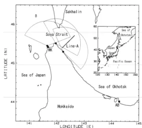
The Sea of Okhotsk (Fig. 1), a marginal sea adjacent to the North Pacific, is one of the southernmost seasonal sea ice zones in the Northern Hemisphere. The Sea of Okhotsk is connected with the Sea of Japan through the Soya/La Perouse Strait, which is located between Hokkaido, Japan, and Sakhalin, Russia. The Soya Warm Current (SWC) enters the Sea of Okhotsk from the Sea of Japan through the Soya Strait and flows along the coast of Hokkaido as a coastal boundary current. It supplies warm, saline water in the Sea of Japan to the Sea of Okhotsk, and greatly affects local climate and marine environment.
However, the SWC has never been continuously monitored due to the difficulties involved in field observations related to various reasons, such as severe weather conditions in winter, political issues at the border strait, and conflicts with high fishing activities. Detailed features of the SWC and its variations have not been clarified. In 2003, we installed three HF ocean radars in the Soya Strait to monitor the surface current fields (Ebuchi et al., 2006). Volume transport of the SWC was estimated using the surface current fields together with current velocity profiles observed by a bottom-mounted acoustic Doppler current profiler (ADCP) (Fukamachi et al., 2008). In this paper, seasonal and subinertial variations in the SWC are investigated by using data from the HF radar, coastal tide gauges and bottom-mounted ADCP.
2.
RESULS
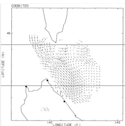
The HF radar measurement was made with an hourly interval and 3 km resolution. To remove the tidal components, a 25-hour running average was applied to the time series of hourly surface current vectors in each grid cell, after which daily mean current fields were calculated. Figure 2 shows an example of the monthly- averaged surface current fields (August 2003). The
Figure 1. A map of the Soya/La Perouse Strait showing locations and coverage of the HF radar stations (NS:
Noshappu, SY: Soya, SR: Sarufutsu), locations of the tide
gauge stations (WK: Wakkanai, AB: Abashiri), and
bottom-mounted ADCP (+).
Figure 2. An example of the monthly averaged surface current vector field after removing wind drift (August 2003).
monthly surface current vector field clearly captures the SWC, which flows from west to east across the Soya Strait and turns southeastward along the coast.
Daily southeastward current components across Line-A (Fig. 1) were averaged monthly and are shown with standard deviations in Fig. 3 for the one-year period from August 2003 to July 2004. The monthly mean profiles showed a clear seasonal variation. The velocity of the SWC reached a maximum of approximately 100 cm/s in summer (August and September) and became weak in winter (January and February). The current axis was located 20 to 40 km from the coast in this region, and the typical width of the SWC was approximately 50 km. In February 2004, there was no offshore data because of sea ice coverage.
Daily surface transport across Line-A (Fig. 1) was defined by the integration of the daily southeastward current component along the line from the coast to a point at which the component becomes negative. Figure 4 shows the time series of the surface transport (thick line).
Note that the unit of surface transport is not volume/time but area/time, because the HF radars provide only the surface current velocity. In winter (from January to March), there often exists lack of data, because the observation region is covered by sea ice.
The driving force of the SWC is ascribed to the sea level difference between the Sea of Japan and the Sea of Okhotsk. For comparison with the surface transport as observed by the HF radars, we calculated the sea level difference between two tide gauge stations, Wakkanai (labeled as WK in Fig. 1) and Abashiri (AB in Fig. 1), which represents sea level difference between the Sea of Japan and the Sea of Okhotsk.
A 48-hour tide-killer filter was applied to the hourly tide gauge records at these stations. The daily-mean sea levels were then calculated, and atmospheric pressure correction was performed using the daily-mean sea level pressure observed at weather stations in the cities of Wakkanai and Abashiri. The time series is shown by a thin line in Fig. 4. The SWC surface transport and the sea level difference along the current show a good correlation with a correlation coefficient of 0.787. Both time series exhibit not only clear seasonal variations but also subinertial variations with time scales of approximately 10 to 15 days. The surface transport and sea level difference oscillated coherently in annual and subinertial time scales.
Figure 3. Monthly-averaged profiles of the southeastward velocity component across Line-A (Fig. 1) with respect to the
distance from the coast from August 2003 to July 2004. Horizontal bars indicate the standard deviations calculated from
daily-averaged velocity profiles.
Figure 4. Daily surface transport of the SWC (thick line) across Line-A and sea level difference between Wakkanai and Abashiri (thin line).
Figure 5 shows variance-preserving spectra of (a) the sea level difference between Wakkanai and Abashiri, (b) surface transport observed by the HF radars, and (c) the near-surface (9-13 m depth) velocity observed by the bottom-mounted ADCP, (d) ECMWF 10-m height wind speed near the strait, (e) coherence and (f) phase of the cross spectrum between the sea level difference and HF radar surface transport, and (g) coherence and (g) phase of the cross spectrum between the ECMWF wind and HF radar surface transport. In the spectra of the (a) sea level difference, (b) surface transport, and (c) near-surface velocity, a broad peak at a frequency ranging from 5 to 20 days representing the subinertial variations was discernible, together with a peak corresponding to the annual cycle. In cross spectrum between the sea level
difference and surface transport, (e) and (f), the coherence was generally high in the frequency band of the subinertial variations around the peak period of 10-15 days, as expected from the time series in Fig. 4. The sea level variations slightly preceded the variations in the surface transport in this frequency range. The cross spectrum between the ECMWF meridional wind and surface transport, (g) and (h), exhibits significant coherence in the subinertial frequency range of 5- to 20- day periods, with a phase lag of one to two days. These results suggest that sea level difference through the strait caused by wind-generated coastally trapped waves on the east coast of Sakhalin and west coast of Hokkaido are considered to be a possible mechanism causing the subinertial variations in the SWC.
Figure 5. Variance-preserving spectra of (a) the sea level difference between Wakkanai and Abashiri, (b) surface
transport observed by the HF radars, and (c) the near-surface (9-13 m depth) velocity observed by the bottom-mounted
ADCP, (d) ECMWF 10-m height meridional wind speed near the strait, (e) coherence and (f) phase of the cross
spectrum between the sea level difference and HF radar surface transport, and (g) coherence and (g) phase of the cross
spectrum between the ECMWF meridional wind and HF radar surface transport.
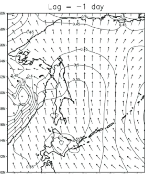
Figure 6. Lag correlation between the ERA-40 wind fields and sea level difference (Wakkanai-Abashiri) from January 1968 to August 2002.Figure placement and numbering.
Figure 6 shows a lag correlation between the ECMWF reanalysis (ERA-40) wind fields and sea level difference for the period from January 1968 to August 2002. The azimuth direction of the wind stress component, which gives the maximum correlation with the sea level difference, is shown by the direction of the arrows, and the maximum correlation coefficient is denoted by the length of the arrows and contours. The maximum value of the correlation coefficient (0.564) was found in the vicinity of the Soya Strait with a one-day lag, implying that the variations in the wind stress field preceded those of the sea level difference by one day. The sea level difference was correlated with meridional wind stress, and southerly winds were observed to increase the sea level difference. This is consistent with the results from the cross spectral analysis shown in Fig. 5.
3.
CONCLUSION
It is clearly demonstrated that the HF radars capture seasonal and subinertial variations in the SWC. The generation mechanism of subinertial variations in the SWC was investigated using data obtained by the HF ocean radars, coastal tide gauges, and a bottom-mounted ADCP, together with wind data from the ECMWF analyses. The results showed that the subinertial variations in the SWC were significantly correlated with the meridional wind stress component over the region.
The subinertial variations in the sea level difference and surface current were delayed from the meridional wind stress variations by one or two days. We concluded that sea level difference through the strait caused by wind- generated CTWs on the east coast of Sakhalin and west coast of Hokkaido are considered to be a possible mechanism casing the subinertial variations in the SWC.
More details concerning the data and their analyses and discussions on the generation mechanism are presented in Ebuchi et al. (2008).
REFERENCES
Ebuchi, N., Y. Fukamachi, K.I. Ohshima, K. Shirasawa, M. Ishikawa, T. Takatsuka, T. Daibo, and M. Wakatsuchi, 2006. Observation of the Soya Warm Current using HF radar. J. Oceanogr., 62(1), pp. 47-61.
Ebuchi, N., Y. Fukamachi, K.I. Ohshima, and M.
Wakatsuchi, 2008. Subinertial, and seasonal and variations in the Soya Warm Current revealed by HF radars, coastal tide gauges, and a bottom-mounted ADCP.
J. Oceanogr. (in press).