Coupled Finite Element Analysis for Semi-implicit Linear and Fully-implicit Nonlinear Scheme in Partially Saturated Porous Medium
Jaehong Kim1 and Richard A. Regueiro2
(Received August 5, 2010 / Revised October 7, 2010 / Accepted October 18, 2010)
ABSTRACT
The paper presents a comparison between a semi-implicit time integration linear finite element implementation and fully-implicit nonlinear Newton-Raphson finite element implementation of a triphasic small strain mixture formulation of an elastic partially saturated porous medium.
The pore air phase pressure pa is assumed atmospheric, i.e., pa = 0, although the formulation and implementation are general to handle increase in pore air pressure as a result of loading, if needed. The solid skeleton phase is assumed linear isotropic elastic and partially saturated
‘consolidation’ in the presence of surface infiltration and traction is simulated. The verification of the implementation against an analytical solution for partially saturated pore water flow (no deformation) and comparison between the two implementations is presented and the important of the porosity-dependent nature of the partially saturated permeability is assessed on comparison with a commercial code for the partially saturated flow with deformation. As a result, the response of partially saturated permeability subjected to the porosity influences on the saturation of a soil, and the different behaviors of the partially saturated soil between staggered and monolithic coupled programs is worth of attention because the negative pore water pressure in the partially saturated soil depends on the difference.
Key words Coupled finite element analysis, Semi-implicit linear, Fully-implicit nonlinear, Partially saturated soil, Consolidation
1) Graduate Student, Dept. of Civil, Environmental, and Architectural Engrg., Univ. of Colorado at Boulder(Corresponding author: [email protected]) 2) Assistant Professor, Dept. of Civil, Environmental, and Architectural Engrg., Univ. of Colorado at Boulder
1. Introduction
A semi-implicit integration scheme leads to a linear solution in time, assuming linear isotropic elasticity for the solid skeleton phase constitutive behavior, and thus is faster computationally and is also easier to implement. A fully-implicit (Backward Euler) time integration leads to a set of nonlinear coupled matrix equations that are solved using Newton-Raphson, and is shown to be more stable for larger time steps, yet slower computationally.
It is assumed the pore air pressure is approximately zero (atmospheric) pa = 0 during loading, although when a surface traction is applied to the ground surface, pore air pressure could play a role (Schrefler and Scotta, 2001; Laloui et al., 2003). We eventually are interested in analyzing the solid soil skeleton deformation and stress coupled to the pore air and water phase pressures to determine potential onset and progressive instability in partially saturated slopes exposed to rainfall infiltration, or other initial boundary value problems involving partially saturated soils.
A coupled hydro-mechanical behavior in triphasic mixture depends on soil hydraulic properties and shear strength properties
affecting the stability of partially saturated slopes. Thus stress changes due to permeability function modify the seepage process because soil hydraulic properties such as porosity, partially saturated permeability and water storage capacity are affected by the changes in stresses (Zhang et al., 2005).
The paper organizes the coupled balance equations, constitutive models, weak form, matrix finite element equations, semi-implicit and fully-implicit nonlinear solution, numerical examples and comparisons with a commercial code for partially saturated porous medium. The good agreement between the obtained results and those from the literature (Srivastava and Yeh, 1991) conforms the reliability and the accuracy of the proposed model.
Finally, the seepage and flow processes in a deformable porous medium with an applied load is solved and results are illustrated.
The comparison of the staggered and monolithic coupled solutions allows to appreciate the influence of the difference between staggered and monolithically coupled anlayses.
2. Balance equations and constitutive equations Mixture theory (Coussy, 2004; de Boer, 2005) starts with the
•
• •
•
•
•
Xl Xg
Yl
Yg
( )l
l X
χ χg( )Xg
( )l
lY
χ
( )g gY χ
( )s
s X
χ
Bl Bg
Bs Bo
l
Bo s
Bo g
Xs
Yg
Yl
x
Xg
Xl
Xs
Yl
Yg
Xs Xl Xg
vs
vl vg
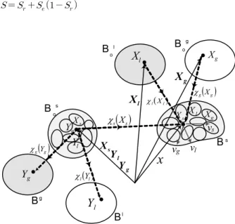
Fig. 1. Mixture theory and solid phase control space for motion of triphasic continuum
concept of volume fraction, , where volume fraction of solid ns, water nw, and air na for general heterogeneous spatial distributions of volume fractions is defined as
(1)
where, is the differential volume of constituent , and dv is the total differential volume (because we assume small deformations, currently there is no distinction between reference and current configurations). The porosity is . Another tenet of mixture theory is to follow the motion of the solid phase, and represent the motion of water and air phases with respect to the solid phase motion, as illustrated in Figure 1. Note in Figure 1 that because the control space is that of the solid phase motion χs(Xs), more than one material point for the liquid (Xl, Yl) and gas (Xg, Yg) phases can flow in and out (by motions χl and χg) of the position held by the solid phase material point Xs. This is classical mixture theory (Coussy, 2004; de Boer, 2005).
Following the formulation in (Borja, 2004), we can write the balance of linear momentum for the mixture, and balance of mass of the water phase as
(2)
(3) where the total stress is written in terms of the effective stress ′
(positive in tension) as ′ , and the degree of saturation, S, is defined as the classical form of van Genuchten (1980),
(4)
(5) where Se is the effective degree of saturation, Sr is the residual degree of saturation, pw is the pore water pressure (positive in compression), and a, n, and m are curve fitting parameters of the soil water characteristic curve (SWCC). The mass density in terms of the partial mass densities , is the gravity acceleration vector, is the superficial Darcy velocity of water with the true velocity of water. The constitutive equations are linear isotropic elasticity for the effective stress, and generalized Darcy’s law (van Genuchten, 1980; Coussy, 2004) for the Darcy velocity of water, written as′ (6)
∇ (7) where ⊗ , the Lamé parameters and ,
∇ is the strain, is the partially saturated permeability, and is the real mass density of water. The permeability is written as
(8)
(9) where is the relative permeability for a partially saturated soil, l is a geometry parameter of dimension length, and is the dynamic viscosity of water.
3. Weak form and nonlinear matrix finite element equations
We assume the whole domain of the body is partially saturated. Applying the method of weighted residuals (Hughes, 1987), we obtain the coupled nonlinear weak form of the balance equations as
∇ ′
(10)
∇
(11)
where is the weighting function for the displacement , is the traction, is the weighting function for the pore water pressure , and is the water seepage positive inward on the
(+) Traction and Infiltration
1m or 3m
1m (-)
Hydrostatic suction profile (Initial condition)
z
1m
or
3m
1m
σ, t
=0 pw 12
•11 •
•
•
•
• •
•
•
• •
•
•
•
•
•
•
•
•
•
•
10
1 2 3
4 5 6
7 8 9
13 14 15
16 17 18
19 20 21
Sw
1
3 2
Fig. 2. Initial condition and three mixed-formulation element mesh
boundary. Assuming a mixed finite element formulation as indicated by the elements in the example mesh in Figure 2, the discretized displacement is interpolated biquadratically (solid nodes in Figure 2), and the pore water pressure bilinearly (open circle nodes in Figure 2).
This leads to a stable spatial integration of the finite element matrix equations, in particular in the nearly incompressible regime (undrained) (Hughes, 1987). Introducing the shape functions, and expressing in matrix form (Hughes, 1987), we may write the coupled nonlinear finite element form as
∧
(12)
∧
(13)
where
∧
is the element assembly operator for element e over number of elements , is the element nodal weighting function values for , is the element nodal weighting function values for , both of which are arbitrary except where they are zero at the boundaries with essential boundary conditions, is the element nodal displacement vector, is the element nodal pore water pressure vector. The internal and external element force vectors, and element stiffness matrices are
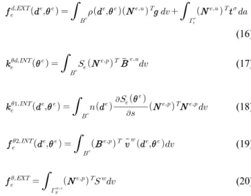
′ (14)
(15)
(16)
(17)
(18)
(19)
(20)
where in general the effective stress governing the solid phase constitutive behavior is a function of displacement (deformation) and pore water pressure (negative suction), where we will assume here it is only a function of displacement (for linear elasticity). is the strain-displacement matrix for
, is a divergence strain-displacement matrix, is the shape function matrix for , is the strain-displacement matrix for , is the shape function matrix for .
After applying boundary conditions, and assembling the finite element equations, the matrix form results as the coupled nonlinear parabolic first order ordinary differential equation to solve
(21) where
For fully-implicit time integration using Backward Euler (Hughes, 1987), we have the coupled nonlinear matrix system of equations to solve via Newton-Raphson
(22) where the equation is evaluated at current time for linearization to solve by Newton-Raphson. A semi-implicit time integration is written as
(23)
Table 1. Material properties of analytical solution
Ks 2.8×10⁻⁶ m/s 1/m 0.45 0.2 2.8×10⁻⁷ m/s 9
0 0.5 1 1.5 2 2.5 3 3.5 4
x 105 -10000
-5000 0
time (sec)
p w (Pa) node#1, top
analytical, top
0 0.5 1 1.5 2 2.5 3 3.5 4
x 105 -6000
-4000 -2000 0
time (sec)
p w (Pa) node#7, middle
analytical, middle
0 0.5 1 1.5 2 2.5 3 3.5 4
x 105 -3000
-2000 -1000 0
time (sec)
p w (Pa) node#13, low
analytical, low
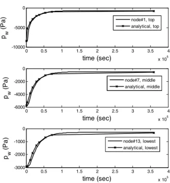
Fig. 3. Fully-implicit nonlinear solution with =1hr
0 0.5 1 1.5 2 2.5 3 3.5 4
x 105 -10000
-5000 0
time (sec) p w (Pa)
0 0.5 1 1.5 2 2.5 3 3.5 4
x 105 -6000
-4000 -2000 0
time (sec) p w (Pa)
0 0.5 1 1.5 2 2.5 3 3.5 4
x 105 -3000
-2000 -1000 0
time (sec) p w (Pa)
node#1, top analytical, top
node#7, middle analytical, middle
node#13, lowest analytical, lowest
Fig. 4. Semi-implicit linear solution with =1hr where ≈ . Each of these equations is
solved for the examples in the next section.
4. Verification for transient partially saturated flow The first example is a verification of the numerical finite element implementation and time integration schemes (semi- implicit versus fully-implicit). To verify, we take the analytical solution of (Srivastava and Yeh, 1991), for water flow through partially saturated porous media with water table pw = 0 at z = 0, and infiltration seepage Sw at z = 1m (Figure 2). After verification, and comparison between semi-implicit linear and fully-implicit nonlinear solution methods, a top traction (Figure 2) is applied to simulate change in pw and downward displacement.
For verification, the constitutive equations for the water phase are modified slightly as follows (Srivastava and Yeh 1991)
(24)
(25)
where Ks is the saturated permeability, is the unit weight of water, is a parameter, is the residual volume fraction of water, and is the saturated volume fraction of water. Note that in (Srivastava and Yeh, 1991) they call their variable is the
“moisture content,” which we refer to as the volume fraction of water . These parameters are shown in Table 1
The initial water infiltration seepage is at zero time (t = 0) and the final (t > 0) water infiltration seepage = 9. The residual degree of saturation is equal to zero (i.e., Se = S) and
= 9800N/m3. The simulation time is 100 hrs. Figure 2 shows the three element mesh with height 1m (or 3m) with initial and boundary conditions for partially saturated flow problem (comparison with analytical solution) and the height 3m is for comparison with commercial code (Seep/w-Sigma/W). All simulations are conducted in plane strain condition (essentially 1 dimensional for the flow problem of (Srivastava and Yeh, 1991), but when the traction is applied in the next example, horizontal stress develops).
The results of our fully-implicit nonlinear and semi-implicit linear finite element solutions are shown in Figures 3 and 4, respectively for a constant time increment of = 1hr. The node number 1, 7, 13 refer, respectively, to pore water pressure nodes on the left hand side of the mesh (open circle nodes) from top, middle, to lowest (the bottom pore water pressure nodes have pw
= 0). The results compare well with the analytical solution (‘x’
mark in figures) of (Srivastava and Yeh, 1991).
The analytical solution is not replicated exactly in closed form in this paper, but the negative pore water pressure values are calculated from the negative water pressure head values from
Figure 1(a) of Srivastava and Yeh(1991)’s paper , and plotted against our finite element solution here. You can see the fully-implicit nonlinear solution in Figure 3 is slightly more accurate (for < 0.5×10⁵) than the semi-implicit linear solution in Figure 4. The difference becomes unnoticeable as the time increment is made smaller →0.
0 0.5 1 1.5 2 2.5 3 3.5 4 x 10⁵ -10000
-5000 0
time (sec) p w (Pa)
0 0.5 1 1.5 2 2.5 3 3.5 4
x 105 -6000
-4000 -2000 0
time (sec) p w (Pa)
0 0.5 1 1.5 2 2.5 3 3.5 4
x 105 -3000
-2000 -1000 0
time (sec) p w (Pa)
node#1, top analytical, top
node#7, middle analytical, middle
node#13, low analytical, low
Fig. 5. Fully-implicit nonlinear solution with =10hr
0 0.5 1 1.5 2 2.5 3 3.5 4
x 105 -10000
-5000 0
time (sec)
p w (Pa) node#1, top
analytical, top
0 0.5 1 1.5 2 2.5 3 3.5 4
x 105 -6000
-4000 -2000 0
time (sec) p w (Pa)
node#7, middle analytical, middle
0 0.5 1 1.5 2 2.5 3 3.5 4
x 105 -3000
-2000 -1000 0
time (sec)
p w (Pa) node#13, lowest
analytical, lowest
Fig. 6. Semi-implicit linear solution with =10hr
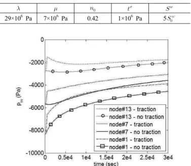
Table 2. Material properties
29×106 Pa 7×10⁶ Pa 0.42 1×10⁶ Pa 5
Fig. 7. profile regarding a traction with =0.05hr To compare the two solution methods, the time increment is
increased to = 10hr in Figures 5 and 6. Beginnings of an oscillation are apparent for the semi-implicit linear method in Figure 6, but it remains stable in the steady-state. For fully-implicit nonlinear, in Figure 5, the solution is smoother.
Comparing CPU times, for = 10hr, it took 9.3 seconds to run the fully-implicit nonlinear solution and 6.6 seconds to run the semi-implicit linear solution, and for = 1hr, it took 28.6 seconds to run the fully-implicit nonlinear solution and 8.2 seconds to run the semi-implicit linear solution.
In general, for smaller time steps, like those needed to resolve a sharp ramp in traction (next example), the semi-implicit linear method is just as accurate as the fully-implicit nonlinear method, but approximately three times as fast. When accounting for elasto-plasticity through the effective stress ′ , a nonlinear solution will be required, and thus it remains to be seen whether a semi-implicit nonlinear solution method will be more efficient computationally than a fully-implicit nonlinear solution.
But this study presents nonlinear elasticity solution for coupled finite element implementation accounting both pore water pressure and traction (external loading) simultaneously.
5. Coupled finite element implementation in deformable soil
The next example considers an application of traction , as depicted in Figure 2. The additional parameters that need to be defined are in Table 2.
The traction is ramped up over 6min, with total simulation time of about 10hrs. Because the time step must be equal to or smaller than 6min to resolve the ramp up of , there is little difference in results between semi-implicit linear and fully-implicit nonlinear solution (we do not use adaptive time-stepping). Thus, we use semi-implicit linear because it is faster. The various with and without traction applied is shown in Figure 7. The node number 1, 7, and 13 are the same nodes with the flow problem in the previous example (e.g., Figure 3). Figure 7 shows that increases upon application of , then decreases as the infiltration water seepage continues to increase the volume fraction of water .
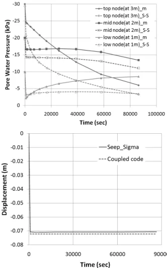
Fig. 8. Displacement at ground surface with traction
Fig. 9. Distribution of and displacement by traction in defor- mable soil
The displacement in Figure 8 shows that without traction there is a small displacement as a result of gravity, while with it there is no noticeable consolidation, although it does increase slightly (becomes more negative) as the excess is dissipated. There could be a build up and dissipation of excess pore air pressure during application of the ground surface traction , but currently
= 0 is assumed. The formulation can be extended to solve for as a separate nodal degree of freedom (Schrefler and Scotta, 2001; Laloui et al., 2003).
In general, many researchers and commercial codes have been used van Genuchten(1980) and Fredlund & Xing(1994)’s functions to predict partially saturated permeability functions.
van Genuchten method of Eq.(26) is the closed form equation to describe the hydraulic conductivity of a soil as a function of soil suction, and Fredlund & Xing’s method of Eq.(27) develops the equation by integrating along the entire curve of the volumetric water content function.
(26)
′
′
(27)
where Ks is saturated hydraulic conductivity, a, n, m are curve fitting parameters, s is soil suction, is the volumetric water content, e is natural number (2.71828), y is a dummy variable of integration representing the logarithm of negative pore water pressure and i, j, N are indices for integration. Both hydraulic conductivities are the function of soil suction or volumetric water content, but these do not consider the porosity of soil.
In Figure 9, the pore water pressures at 3, 2, 1m are the results from the same nodes of previous numerical examples. In order to compare the pore water pressure (or matric suction) in deformable soil column, Sigma/W is used together with Seep/W to perform a staggered coupled consolidation analysis in the mesh (3m height) as shown in Figure 2. The commercial code (Geo-slope, 2007) used the partially saturated permeability of van Genuchten method in Eq.(26). Our monolithically coupled code used the partially saturated permeability of Eqs.(8) and (9) considering dependence on porosity as well as matric suction. It considers that solid skeleton’s behavior by external loading influences partially saturated permeability in each time step. The effect of porosity produced a small difference of pore water pressure according to the passage of time as shown in Figure 9.
The analysis of coupled Seep/W and Sigma/W is performed in a staggered manner separately.
Staggered coupled analysis estimates individually for seepage and stress analysis, namely, after completing seepage and flow process in rigid soil body in Seep/W, Sigma/W is formulated for soil deformation using results obtained from Seep/W. However, monolithic coupled analysis can describe that pore water pressure
change due to seepage leads to changes in stresses and to deformation of a soil. Similarly, stress changes modify the seepage process since soil hydraulic properties such as porosity, permeability and water storage capacity are affected by the changes in stresses. Hence a monolithically coupled hydro- mechanical model is preferred to analyze the behavior and stability of a partially saturated soil subjected to external loads, especially rainfall. As a result, the seepage and stress-deformation problems should be linked simultaneously.
When traction is applied at the first time step, water flow causes a compacted soil obtained from Sigma/W to be saturated quickly. Both displacements on ground surface is similar because of using the same elastic moduli.
6. Conclusions
For a general nonlinear finite element formulation and implementation at small strain, the main contribution of this paper is to compare a fully-implicit nonlinear finite element solution to a semi-implicit linear finite element solution. It was found that for large time steps, the fully-implicit scheme is more stable and accurate, but for practical nonlinear finite element analyses requiring smaller time increments to resolve the solution more accurately, a semi-implicit linear scheme is more computationally efficient.
The other contribution is to implement the partially saturated permeability with the function of degree of saturation S and porosity n for seepage analysis in a deformable soil. When both seepage and traction are applied to the top surface of soil column, the seepage and flow processes in a deformable soil are influenced by solid skeleton deformations. Similarly, stress changes will modify the seepage process since soil hydraulic properties such as porosity and permeability are affected by the changes in stresses. By identifying difference between results of both codes (Seep/W-Sigma/W and my own code), it essentially revealed that the difference of analyses through flow-deformation
mechanism might play an important role on hydraulic pattern of partially saturated soils.
References
1. Coussy, O. (2004). Poromechanics. John Wiley & Sons.
2. de Boer, R. (2005). Trends in Continuum Mechanics of Porous Media: Theory and Applications of Transport in Porous Media.
Springer.
3. Borja, R.(2004). “Cam-Clay Plasticity. Part V: A Mathematical Framework for Three-phase Deformation and Strain Localization Analyses of Partially Saturated Porous Media”, Computer Methods in Applied Mechanics and Engineering, 193, 5301-5338.
4. GEO-SLOPE. (2007). Version 7.13. User’s guide, International Ltd., Calgery, Canada.
5. Fredlund, D.G. and Xing, A. (1994). “Equations for the soil- water characteristic curve”, Canadian Geotechnical Journal, 31, 521-532.
6. Hughes, T. J. R. (1987). The Finite Element Method. Prentice- Hall: New Jersey.
7. Laloui, L., Klubertanz, G., and Vulliet, L. (2003). “Solid-liquid- air coupling in multiphase porous media”, International Journal for Numerical and Analytical Methods in Geomechanics 27(3), 183-206.
8. Lu, N. and Likos, W. (2004). Unsaturated Soil Mechanics. Wiley.
9. Schrefler, B., and Scotta, R. (2001). “A fully coupled dynamic model for two-phase fluid flow in deformable porous media”, International Journal for Numerical and Analytical Methods in Geomechanics, 20, 785-814.
10. Srivastava, R. and Yeh, T.-C. J. (1991). “Analytical solutions for one-dimensional, transient infiltration toward the water table in homogeneous and layered soils”, Water Resources Research, 27(5), 753-762.
11. van Genuchten, M. (1980). “Closed-form equation for predicting the hydraulic conductivity of unsaturated soils”, Soil Science Society of America Journal 44(5), 892-898.
12. Zhang, L.L., Zhang, L.M., and Tang, W.H. (2005). “Rainfall- induced slope failure considering variability of soil properties”, Geotechnique, 55(2), 183-188.