1. Introduction
Coulomb proposed a method for the determination of active earth pressures that included the effect of friction between soil and wall (Coulomb, 1776). In this method, a linear failure surface was assumed and force equilibrium condition was applied. In order to evaluate the maximum active earth pressure, several trial failure surfaces were tried and the one producing the critical force was selected.
Especially, Coulomb’s solution for active earth pressure refers to the earth pressure due to the soil weight only.
However, in many practical problems, the lateral earth pressure was due to not only soil weight but also applied external loads i.e. line load and uniform load. If external
loads are applied, the time consuming Culmann’s graphical method (1875) was usually applied because Coulomb’s method cannot provide analytical solution. With this graphical method, the procedure of estimating active earth pressure is not only complicate and cumbersome but also inaccurate. Another defect of Coulomb’s active earth pressure formula is that soil cohesion and adhesion were not considered in its original derivation. As it is well known, the shear strength of soil is measured in terms of two soil parameters i.e. cohesion and soil friction angle. Grain crushing, resistance to rolling and other factors are implicitly included in these two parameters (Bowles, 1988). Therefore, since Coulomb’s active earth pressure formula also cannot consider soil cohesion value, the active earth pressure value by Coulomb’s formula will be conservative.
Generalized Formula for Active Earth Pressure Estimation with Inclined Retaining Wall
점착력을 고려한 배면 경사 옹벽에서의 주동토압 산정 공식
Kim, Woncheul1) ・ Hwang, Youngcheol† 김 원 철 ・ 황 영 철
ABSTRACT :Active earth pressure formula, which can consider the effects of ground surface inclination, inclination of inside retaining wall face, wall friction, line load, uniform load, soil cohesion and adhesion, was derived based on the force equilibrium principle.
In order to verify the accuracy of this proposed formula, the calculated active earth pressures by the proposed formula were compared with those of graphical solutions. Also, the active earth pressures determined by the proposed formula were compared with those by Coulomb’s, Rankine’s and Mazindrani’s solution under specific conditions. The results matched quite well not only with the graphical solutions but also with those by three other methods. Also, the trend of active earth pressures by the proposed formula were corresponded with results of experimental study by Fang, et al. It can be concluded that this generalized formula not only can overcome the limitations of Rankine’s, Coulomb’s and Mazindrani’s active earth pressure formula but also can consider the external loading conditions.
Keywords : Active earth pressure, Cohesion, Adhesion, External loading conditions
요 지 : 본 논문에서는 지표면 경사각 벽면 경사각 벽면 마찰각 선하중 등분포하중 점착력 부착력의 영향을 고려할 수 있는, , , , , ,
주동토압공식을 힘의 평형이론을 근거로 도출하였다 이 제안식의 정확성을 검증하기 위하여 도해법에 의해 산정된 토압과 비교하. ,
였으며, Coulomb, Rankine, Mazindrani 공식에 의한 산정 결과와도 비교하였다 산정 결과는 도해법 결과뿐만 아니라. Coulomb,
공식의 가지 방법에 의한 결과와 잘 일치되었다 또한 제안식에 의한 주동토압은 등의 실험연구 결과와
Rankine, Mazindrani 3 . , Fang
일치하는 경향을 나타내었다 이 일반화된 공식은. Coulomb, Rankine, Mazindrani의 주동토압공식의 한계를 극복할 수 있을 뿐만 아니라 외부하중조건을 고려할 수 있는 것으로 평가되었다.
주요어 : 주동토압 점착력 부착력 외부하중조건, , ,
1) 정회원, WonGeo E&C대표이사 공학박사, 한국지반환경공학회 논문집 제 권 제 호9 5 2008년 월6 pp. 71~81
Rankine (1857) suggested a method for the determination of earth pressure applying essentially the same assumptions as Coulomb’s but zero wall friction is assumed and soil cohesion is considered. However, according to Sherif et al.
(1982), friction between wall and soil is one of the important parameters for active earth pressure evaluation. The other limitations of original Rankine’s method are that the slope of ground surface should be horizontal and the inclination of inside wall face should be vertical with cohesive backfilled soil condition. Another formula, which can be applied to the inclined ground surface case with granular backfilled soil, is available but this formula cannot be applied if the soil friction angle is larger than the ground surface inclination.
Therefore, since this formula is not practical or cannot be applied to cohesive backfilled soil, the original Rankine formula was used for discussion in this paper. However, in real world, the retaining wall usually has inclined ground surface and inclined inside wall face under cohesive backfilled soil condition. Therefore, in such case, Terzaghi’s (1943) graphical approach is usually applied for evaluation of active earth pressure. However, this procedure becomes tiresome for solving practical retaining wall problems because several Mohr circle should be tried to determine the lateral earth pressure. In order to eliminate these inconveniences, Mazindrani and Ganjali (1997) developed a method that can be applied to cohesive soil with inclined surface cases. Since Mazindrani’s formula for active earth pressure is developed based on the Rankine theory, this approach has the same limitations with Rankine’s such that wall friction was assumed zero and the inclination angle of inside wall face should be vertical.
Moreover, if external loads are applied with inclined ground slope condition, Rankine’s and Mazindrani’s methods cannot be applied for the estimation of active pressure and graphical approach is the only solution up to now.
Significant and valuable studies associated with earth pressure have been carried out by Terzaghi (1932), Schofield (1961), Mackey and Kirk (1967), Matteotti (1970), Bros (1972), Sherif and Mackey (1977), Sherif et al. (1982), Sherif et al. (1984), Duncan et al. (1991) and other researchers and most of the study was concerned with horizontal ground surface. Fortunately, Fang et al. (1997) studied lateral earth pressure of dry sand with inclined ground surface through the experimental research. Based on their experimental data, it has been found that the active and passive earth pressures
for various backfill sloping angles are in good agreement with the values determined by Coulomb and Terzaghi’s solution. They also found that Rankine’s solution tends to overestimate the active earth pressure if inclined ground surface angle is less than 20°. Finally, they concluded that Rankine theory might not be appropriate to determine either active or passive earth pressure against a rigid wall with sloping backfill. Unfortunately, if the geotechnical engineer should design the retaining wall that has inclined ground surface, inclined wall face and external loads under cohesive soil condition, the estimation of active earth pressure was remained problematic.
In this paper, a generalized active earth pressure formula has been developed based on the force equilibrium condition and this formula can consider cohesion, adhesion, wall friction, inclination of inside wall face, ground surface inclination, and external loads. For the verification of this proposed formula, the active earth pressure values are compared with those of graphical and theoretical solutions from the published literatures.
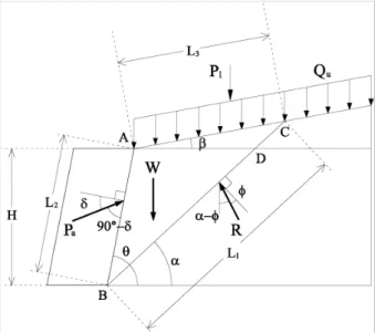
2. Analysis of Acting Forces Around Assumed Failure Wedge
The basic assumptions for the active earth pressure estimation are: the soil is homogeneous, the mode of failure plane is linear, all external loads are applied at the inside failure wedge and the length of applied uniform load is long
Fig. 1. General Scheme for Active Earth Pressure Estimation.
enough to be intersected by the failure plane. The general scheme for active earth pressure is shown in Fig. 1. For convenience, positive sign was assigned for downward and rightward movement, and negative sign was assigned for upward and leftward movement.
There are seven forces that act around assumed failure wedge ABC and these are included in Fig. 1. As mentioned before, since this formula is driven based on the force equilibrium, these forces should be divided into components of x and y directions in order to apply the force equilibrium principle. Therefore, these seven forces are divided into x and y component as follows.
The soil weight of assumed failure triangle wedge ABC denoted by W acts to the gravitational direction and has no horizontal force. The line load denoted by Pl and uniform load denoted by Qu also act to the gravitational direction, therefore, have no horizontal forces. In Fig. 1, since the general geometry of retaining wall may have slope, the inclination angle is denoted by .
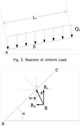
As shown in Fig. 2, the length of uniform load denoted by L3 will be changed with the variation of wedge failure angle denoted by , which is defined the angle between failure plane of wedge and bottom horizontal line. Since value is function of many other factors, detailed derivation
of general equation for L3 will be discussed later.
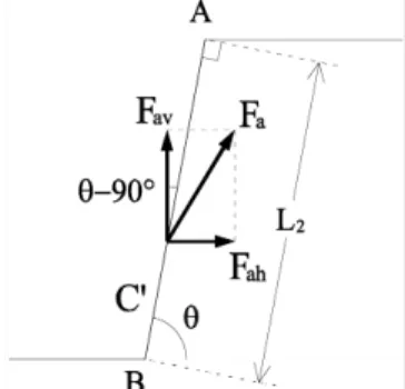
With the same principle, soil reaction denoted by R can be divided into vertical force denoted by Rvand horizontal force denoted by Rh. As shown in Fig. 3, these vertical and horizontal components of soil reaction can be expressed as Rv = ‒ R cos ( ‒ ) and Rh = ‒ R sin ( ‒ ), respectively. The negative signs mean downward movement with vertical component and leftward movement with horizontal component, respectively.
The active earth pressure denoted by Pa can be divided into vertical force denoted by Pav and horizontal force denoted by Pah. As shown in Fig. 4, is geometrical inclination of inside wall face and is friction angle between wall and soil. Applying these symbols, the vertical and horizontal components of active earth pressure can be expressed as Pav =‒ Pasin ( ‒ 90° + ) and Pah = Pa cos ( ‒90° + ), respectively. The negative sign means downward movement with vertical component and the positive sign means rightward movement with horizontal component, respectively.
The resistance due to soil cohesion denoted by C can be divided into vertical force denoted by Fcv and horizontal force denoted by Fch. These vertical and horizontal components
Fig. 2. Reaction of Uniform Load.
Fig. 3. Reaction of the Soil.
Fig. 4. Reaction of Active Earth Pressure.
Fig. 5. Reaction of Cohesion Force.
of resistance force by soil cohesion can be expressed as Fcv
= ‒ C L1 sin and Fch = C L1 cos , respectively. As shown in Fig. 5, the length of failure line denoted by L1is the function of failure angle denoted by . As it is mentioned,
value is function of many other factors, the derivation of general equation for L1will be discussed later. The negative and positive signs with each formula mean upward movement with vertical component and rightward movement with horizontal component, respectively.
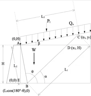
Wall adhesion develops from any cohesion in soil (Bowels, 1988), therefore, adhesion is defined as the adhesive force between the wall and backfilled soil due to soil cohesion only. Resistance due to soil adhesion denoted by C can be′ divided into vertical force denoted by Fav and horizontal force denoted by Fah. These vertical and horizontal components of resistance force by adhesion can be expressed as Fav =
C L
‒ ′ 2sin (180° ‒ ) and Fah = ‒ C L′ 2cos (180° ‒ ), respectively. As shown in Fig. 6, L2 is the length of inside wall face which contacts with soil and is the inclination of inside wall face. The negative sign with each formula
means upward movement with vertical component and leftward movement with horizontal component, respectively. The discussed vertical and horizontal forces are summarized in Table 1.
In order to satisfy the force equilibrium principle, Σ FV
= 0 andΣFH= 0 conditions should be achieved. Therefore, from the Σ FV = 0 condition and Table 1, following equation can be driven:
90 ) sin(
P ) cos(
R L Q P W
0= + l+ u 3− α−φ − a θ− o+δ 180 )
sin(
L ' C sin
CL1 α− 2 o−θ
− (1)
Above formula can be rearranged as following equation, 90 )
sin(
P L Q P W ) cos(
R α−φ = + l+ u 3− a θ− o+δ 180 ) sin(
L ' C sin
CL1 α− 2 o−θ
− (2)
From the Σ FH = 0 condition and Table 1, following equation can be driven:
90 ) cos(
P ) sin(
R
0=− α−φ + a θ− o+δ 180 ) sin(
L ' C cos
CL1 α− 2 o−θ
− (3)
Above formula can be rearranged as following equation, 90 )
cos(
P ) sin(
R α−φ = a θ− o+δ
180 ) cos(
L ' C cos
CL1 α− 2 o−θ
+ (4)
In order to get rid of soil reaction R, Eq. (4) was divided by Eq. (2) and following relationship is driven.
) tan(α−φ
) 180 sin(
L C sin CL ) 90 sin(
P L Q P W
) 180 cos(
L C cos CL ) 90 cos(
P
2 1
a 3 u l
2 1
a
θ
−
′ °
− α
− δ +
°
− θ
− + +
θ
−
′ °
− α + δ +
°
−
= θ Fig. 6. Reaction of Adhesion Force. (5)
Table 1. Summary of Acting Forces Around Soil Wedge
Description Vertical Forces Horizontal Forces
1 Weight of Wedge
W (F/L) W 0
2 Line Load
Pl (F/L)
Plv
Pl
Plh
0
3 Uniform Load
Qu(F/L2)
Quv
QuL3
Quh
0
4 Soil Reaction
R (F/L)
Rv
‒R cos ( ‒ )
Rh
‒R sin ( ‒ ) 5 Active Earth Pressure
Pa(F/L)
Pav
‒Pasin ( + ‒ 90°)
Pah
Pa cos ( + ‒ 90°)
6 Cohesion
C (F/L2)
Fcv
‒C L1sin
Fch
C L1cos
7 Adhesion
C (F/L′ 2)
Fav
‒C L′ 2sin
Fah
C L′ 2cos
Eq. (5) can be rearranged as following form,
⎪⎭
⎪⎬
⎫
⎪⎩
⎪⎨
⎧
θ
− +
α
− φ
− α θ
−
−
φ
− α α
− φ
− α +
φ
− α + φ
− α
⎭ ×
⎬⎫
⎩⎨
⎧
δ +
− θ + φ
− α δ +
−
= θ
180 ) cos(
L ' C cos CL ) tan(
180 ) sin(
L ' C
) tan(
sin CL ) tan(
L Q ) tan(
P ) tan(
W
90 ) cos(
) tan(
90 ) sin(
P 1
2 o o 1
2
1 3
u l
o a o
(6) The terms of this equation can be classified into as soil weight, external load, soil cohesion and adhesion. For convenience, let soil weight term is S, external load term is T, soil cohesion term is U and adhesion term is V. Then Eq. (6) can be expressed as follow.
(S T U V)
90 ) cos(
) tan(
90 ) sin(
Pa o 1 o + + +
⎭⎬
⎫
⎩⎨
⎧
δ +
− θ + φ
− α δ +
−
= θ
(7) Where,
180 ) cos(
L ' C ) tan(
180 ) sin(
L ' C V
cos CL ) tan(
sin CL U
) ( L Q ) tan(
P T
) tan(
W S
2 o 2 o
1 1
3 u l
θ
− +
φ
− α θ
−
−
=
α
− φ
− α α
−
=
φ
− α +
φ
− α
=
φ
− α
=
3. The Derivation of General Equation for L1, L2 and L3
Above formulas include unknown terms i.e. W, , L1, L2
and L3 and these unknown terms are evaluated as follows.
As shown in Fig. 7, and are known values from the geometric condition. Therefore, the intersection points A,
B, C, D, and E can be defined as x-y coordinate form i.e.
A(0, H), B(L2 cos (180° ‒ ), 0), C(X3, Y3), D(X2, H) and E(0,0). With these defined coordinates of intersection points, the equations of line BC, AD and AC can be defined as following forms, respectively i.e. F (X, Y)1 = (tan ) X + C3, F (X, Y)2 = H and F (X, Y)3 = (tan ) X + H.
Based on above discussion and Fig. 7, the length of wall L2 can be expressed as following equation.
) 180 sin(
L2 H
θ
−
= °
(8) As shown in Fig. 7, since point B is on the Line BC, the values of point B should satisfy following equation F (X, Y)1= (tan ) X + C3. Therefore, substitute the values of point B into the equation of line BC. Then, following relationship is driven i.e. C3=‒ (tan) {L2cos (180° ‒ )}.
Substitute C3 value into equation of line BC. Then the equation of line BC can be expressed as following form.
{L cos(180 )}
) (tan X ) (tan ) Y , X (
F 1= α − α 2 o−θ (9)
Since point D is on the line BC, H = (tan) X2‒(tan){L2
cos (180° ‒ )} condition should be satisfied. Therefore,
α
θ
−
° α
= +
tan
) 180 cos(
L ) (tan
X2 H 2 (10)
From the Fig. 7, the line BC and line AC meet at point C. Therefore, following relationship should be satisfied.
{L cos(180 )}
) (tan X ) (tan H X )
(tanβ 3+ = α 3− α 2 o−θ (11)
Rearrange Eq. (11) in term of X3 and the value of X3
can be as follow.
β
− α
θ
−
° α
= +
tan tan
) 180 cos(
L tan
X3 H 2
(12) Substitute X3into equation of line AC i.e. F (X, Y)3= (tan
) X + H and the value of Y3 can be expressed as follow.
tan H tan
) 180 cos(
L tan tan H
Y3 2 +
⎭⎬
⎫
⎩⎨
⎧
β
− α
θ
−
° α
β +
= (13)
With applying all above derived relationships, W, L1and L3 can be expressed in terms of .
⎥⎦
⎢ ⎤
⎣
⎡
β
− α
θ
−
° α
+ β
⎭⎬
⎫
⎩⎨
⎧
α θ
−
° α γ + +
α
−
° γ +
°
− θ γ
=
tan tan
)}
180 cos(
L tan H { tan tan
) 180 cos(
L tan H 2 1
) 90 tan(
2 H ) 1 90 sin(
L 2 H W 1
2 2
2 2
Fig. 7. Coordinates of Point A, B, C, D and E. (14)
⎥⎦
⎢ ⎤
⎣
⎡ +
β
− α
θ
−
° α
+ β
= α
= α H
tan tan
)}
180 cos(
L tan H { tan sin
1 sin
L1 Y3 2
(15)
⎭⎬
⎫
⎩⎨
⎧
β
− α
θ
−
° α
+
= β
= β
tan tan
) 180 cos(
L tan H cos
1 cos
L3 X3 2
(16) Substitute Eq. (14), (15) & (16) into Eq. (7) and soil weight term S, external load term T, soil cohesion term U and adhesion term V can be written as following forms, respectively.
Soil Weight Term
) 90 ) tan(
180 sin(
) 90 H sin(
2 1
S 2⎢ o o
⎣
⎡ + °−α
θ
−
− γ θ
=
tan
) 180 cot(
tan 1
⎭⎬
⎫
⎩⎨
⎧
α θ
−
° α
+ +
× tan ( )
tan tan
)}
180 cot(
tan 1 {
tan ⎥ α−φ
⎦
⎤
⎭⎬
⎫
⎩⎨
⎧
β
− α
θ
−
° α
+ β
(17)
External Load Term
) tan tan(
tan
) 180 cot(
tan H 1 Q ) tan(
P
T l u α−φ
⎭⎬
⎫
⎩⎨
⎧
β
− α
θ
−
° α + +
φ
− α
= (18)
Soil Cohesion Term
⎥⎦
⎢ ⎤
⎣
⎡ +
β
− α
θ
−
° α + β
− α
= 1
tan tan
)}
180 cot(
tan 1 { tan sin U H
{Csinαtan(α−φ)+Ccosα} (19)
Adhesion Term
{C'sin(180 )tan( )
) 180 sin(
V H °−θ α−φ
θ
−
− °
=
}
) 180 cos(
'
C °−θ
− (20)
Substitute Eq. (17), (18), (19) & (20) into Eq. (7) and then the proposed formula can be expressed as following.
{ } { }
⎥⎥
⎥⎥
⎥⎥
⎥⎥
⎥⎥
⎥⎥
⎥⎥
⎥⎥
⎥
⎦
⎤
⎢⎢
⎢⎢
⎢⎢
⎢⎢
⎢⎢
⎢⎢
⎢⎢
⎢⎢
⎢
⎣
⎡
θ
−
°
− φ
− α θ
− θ °
−
− ° α + φ
− α α
⎟⎟×
⎠
⎜⎜ ⎞
⎝
⎛ +
β
− α
θ
−
° α + β
− α φ
−
⎟⎟ α
⎠
⎜⎜ ⎞
⎝
⎛
β
− α
θ
−
° α +
+ φ
− α + φ
−
⎭ α
⎬⎫
⎟⎟⎠
⎜⎜ ⎞
⎝
⎛
β
− α
θ
−
° α + β
⎩⎨
⎧ ⎟×
⎠
⎜ ⎞
⎝
⎛ α
θ
−
° α + + α
−
° θ+
−
°
− γ θ
⎭×
⎬⎫
⎩⎨
⎧
δ +
°
− θ + φ
− α δ +
°
−
= θ
) 180 cos(
' C ) tan(
) 180 sin(
' )C 180 sin(
cos H C ) tan(
sin C
tan 1 tan
)}
180 cot(
tan 1 { tan sin ) H tan tan(
tan ) 180 cot(
tan H1 Q
) tan(
P ) ( tan tan
tan
)}
180 cot(
tan 1 { tan
tan ) 180 cot(
tan ) 1 90 ) tan(
180 sin(
) 90 H sin(
2 1
) 90 cos(
) tan(
) 90 ( sin P 1
u
l o
2 a
(21)
The parameters, which are included in Eq. (21), are known values from wall geometry or soil properties except assumed wedge failure angle . Therefore, the maximum active earth pressure Pa can be evaluated with changing values.
4. The Comparison of Active Earth Pressure Among the Original Coulomb, Rankine’S and Proposed Formular
The original Coulomb and Rankine’s active earth pressures were expressed as following equations, respectively (Taylor, 1956).
{ } { }
2 2
a sin( ) sin( )sin( ) /sin( )
) sin(
H csc 2 P 1
⎥⎥
⎦
⎤
⎢⎢
⎣
⎡
β
− θ β
− φ δ + φ + δ + θ
φ
− θ γ θ
= (22)
⎟⎠
⎜ ⎞
⎝
⎛ °−φ
⎟−
⎠
⎜ ⎞
⎝
⎛ °−φ γ
= 2CHtan 45 2
45 2 tan 2 H Pa 1 2 2
(23) The active earth pressure of cohesionless soil with inclined ground surface by Rankine was expressed as following equation (Taylor, 1956).
⎪⎭
⎪⎬
⎫
⎪⎩
⎪⎨
⎧
φ
− β + β
φ
− β
− β β γ
= 2 2
2 2 2
a cos cos cos
cos cos cos cos
2 H P 1
(24)
The direct comparisons of Eq. (21), (22), (23) and (24) are not possible because each formula has its own distinctive form. For comparison purpose, the same conditions, which can be applied to both Coulomb and Rankine’s active earth pressure formula, are applied to the proposed formula. Since no cohesion, adhesion, external load are considered for Coulomb’s active earth pressure formula, the proposed formula can be reduced as Eq. (25).
) 90 cos(
) tan(
) 90 sin(
) tan(
Pa W
δ +
°
− θ + φ
− α δ +
°
− θ
φ
−
= α
(25) In order to reflect the limitations of Rankine’s active earth pressure formula, = 90°, = 0 condition are applied to Eq. (14) and the reduced formula is shown in Eq. (26).
) 90 tan(
2 H
W=1γ 2 °−α (26)
Substitute Eq. (26) into Eq. (25), then the proposed
active earth pressure formula can be expressed as follow.
⎭⎬
⎫
⎩⎨
⎧
δ +
°
− θ + φ
− α δ +
°
− θ
φ
− α α
− γ °
= sin( 90 )tan( ) cos( 90 )
) tan(
) 90 H tan(
2 Pa 1 2
(27)
If the same conditions are applied to Eq. (21), (22), (23), (24) and (27), the active earth pressures values should be same. Because of the limitations of each formula, = 90°
was applied and zero values were assigned to C, C ,′ and
. When = 17.4 kN/m3, = 26°, C = 0, H = 6 m, C′
= 0, = 90°, = 0 and = 0° are applied to Eq. (21), (22), (23), (24) and (27), the active earth pressure of all the five equations are exactly same and the value is 122.293 kN/m with failure angle = 58°. This failure angle can be determined by proposed formula only.
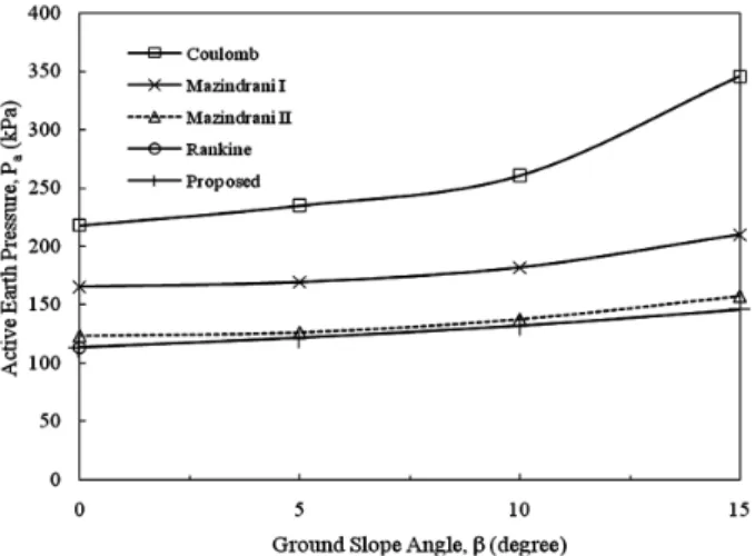
With original Rankine formula, wall friction = 0° was assumed. However, in reality, most retaining walls are far from frictionless. Generally, one half or two third of soil friction angle is used for design if Coulomb formula is applied. In order to find the effect of wall friction, all the same values but = 17° are applied to Eq. (22), and (27) and the active earth pressures are exactly same value of 108.83 kN/m with failure angle = 54°. Based on the above comparison, neglecting wall friction value is not only unreasonable but also great loss.
5. Verification of Proposed Formular
In order to verify the accuracy of the proposed formula, the active earth pressures by proposed formula were compared with those by graphical approach. These are from Bowles
(1988), Das (1984), Dunn et al. (1980), Suton (1975), Prakash (1981), Peck et al. (1974), Taylor (1956), Terzaghi (1943), Terzaghi and Peck (1948), Lamb and Whitman (1979) and Venkatramaiah (1993). These eleven comparison results are summarized in Table 2 and among them, active earth pressure of retaining walls with line load, with no external load and with uniform load under inclined ground surface condition are discussed through case number 2, 7 and 9, respectively.
The active earth pressure by proposed formula is compared with result of Culmann’s graphical method under cohesive soil condition at case No. 10. At the subtitle of the comparison with Rankine theory, the active earth pressure by proposed formula is compared with that by Mazindrani and Ganjali (1997) method.
Case No. 2 (Line Load)
A 3.5 m high retaining wall of which ground surface inclination = 0° and 10 kN/m of line load (Pl) was applied 2 m behind on the top of wall. From the given conditions, unit weight of soil = 15.6 kN/m3, friction angle of soil = 32°, inside wall face inclination = 90°
and wall friction angle = 20° and soil cohesion C = 0 are used (Dunn et al., 1980). The published Pa value by Culmann’s graphical method was Pa = 31 kN/m and the solution obtained by the proposed formula i.e. Eq. (21) is Pa = 30.906 kN/m, with failure angle = 61°.
Case No. 7 (Rebhann s Graphical Method)’ A 5.0 m high retaining wall of which ground surface slope = 10° and no external loads are applied. From the
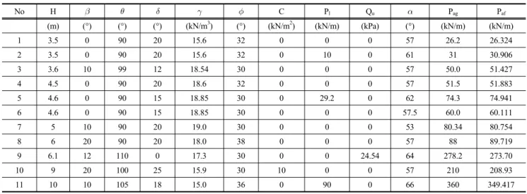
Table 2. Comparison of Active Earth Pressures Determined by Graphical, Theoretical Solution and Proposed Formula
No H C Pl Qu Pag Paf
(m) (°) (°) (°) (kN/m3) (°) (kN/m2) (kN/m) (kPa) (°) (kN/m) (kN/m)
1 3.5 0 90 20 15.6 32 0 0 0 57 26.2 26.324
2 3.5 0 90 20 15.6 32 0 10 0 61 31 30.906
3 3.6 10 99 12 18.54 30 0 0 0 57 50.0 51.427
4 4.5 0 90 20 18.6 32 0 0 0 57 51.5 51.883
5 4.6 0 90 15 18.85 30 0 29.2 0 62 74.3 74.941
6 4.6 0 90 15 18.85 30 0 0 0 57.5 60.0 60.111
7 5 10 90 20 19.0 30 0 0 0 53 80.34 80.754
8 6 20 90 20 18.0 38 0 0 0 57 88 89.719
9 6.1 12 110 0 17.3 30 0 0 24.54 64 278.2 273.70
10 9 20 100 25 15.9 30 10 0 0 57 210 208.93
11 10 10 105 18 15.0 36 0 90 0 66 360 349.417
given conditions, unit weight = 19.0 kN/m3, friction angle of soil = 30°, wall inclination = 90° and wall friction angle = 20° are used (Venkatramaiah, 1993). The published Pavalue by Rebhann’s graphical method is 80.34 kN/m and the solution obtained by the proposed formula was 80.754 kN/m, with failure angle = 53°.
Case No. 9 (Uniform Load)
A 6.1 m high retaining wall, which has a ground surface slope = 12° and applied uniform load Qu= 24.54 kN/m2, is analyzed. From the given conditions, soil unit weight
= 17.3 kN/m3, soil friction angle = 30°, wall inclination
= 110° and wall friction angle = 0° are used (Lamb and Whitman, 1979). The published solution is Pa = 278.22 kN/m, the solution obtained by the proposed formula is Pa
= 273.70 kN/m, with failure angle = 57°. As it was mentioned by Lamb and Whitman (1979), the published solution was approximated value, therefore, there is a little differences between the published value and that determined by the proposed formula.
Case No.10 (Cohesion)
As mentioned, this proposed formula can consider cohesion (C) and adhesion (C ) values based on the force equilibrium′ principle. Therefore, the active earth pressure with cohesive backfilled soil was estimated by proposed formula and it was compared with that of graphical solution. From the given conditions, wall height H = 9 m, slope inclination at the top of wall = 20°, unit weight of soil = 15.9 kN/m3, friction angle of soil = 30°, wall inclination = 100° and wall friction angle = 25°, soil cohesion C = 10 kN/m2and adhesion between wall and soil C = 0 are used′ (Suton, 1975). The published Pavalue by Culmann’s graphical method was Pa = 210 kN/m and the solution obtained by the proposed formula is Pa = 208.930 kN/m, with failure angle = 57°.
The Comparison with Rankine Theory
The original Rankine’s active earth pressure formula cannot be applied if the retaining wall has inclined ground surface and backfilled soil is cohesive. Therefore, Mazindrani and Ganjali (1997) developed a method that can estimate the
active earth pressure of cohesive soil with inclined surface.
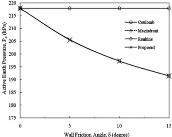
This method can consider the effect of tension crack that can be developed just behind the top of retaining wall. In this example, the solutions developed by Mazindrani and Ganjali (1997) are compared with the solutions by proposed formula. From the given conditions, the wall height H = 6.5 m, slope inclination at the top of wall = 5°, unit weight of soil = 17.52 kN/m3, friction angle of soil = 15°, inside wall face inclination = 90° and wall friction angle = 0°, soil cohesion C = 10.5 kN/m2 and adhesion between wall and soil C = 0 are applied (Mazindrani and′ Ganjali, 1997). The active earth pressure by the Mazindrani method is 124.7 kN/m with 1.56 m tension crack at the top of retaining wall whereas the active earth pressure by proposed formula is 121.505 kN/m. As it is shown, the active earth pressure by the proposed formula was less than that of Mazindrani’s method. Besides this numerical difference, there is another difference i.e. the active earth pressure by proposed formula is under no tension cracked condition. If the tension crack was not developed, the active pressure by Mazindrani method is 164.06 kN/m.
This difference was corresponded with the results of experimental research by Fang et al. (1997). They carried out interesting experimental study with dry sand under = 90,
> 0 conditions and the experimental active earth pressure values have good agreement with the values determined by Coulomb and Terzaghi’s theory. They also showed that Rankine formula overestimate the active earth pressure if the inclination slope of backfill is smaller than 20° and they concluded that the active earth pressure by Rankine theory may not appropriate for the lateral earth pressure estimation. After Mazindrani and Ganjali (1997), the estimation of active earth pressure with inclined surface is possible but this formula still has limitations i.e. wall friction should be zero, wall inclination should be 90° and external loads cannot be considered. With the same problem, if friction angle between the wall and soil is assumed 7°, the active earth pressure with the proposed formula is Pa= 104.43 kN/m.
The active earth pressures by graphical method and proposed formula are summarized in Table 2 and Pag and Paf represent active earth pressure by graphical method and proposed formula, respectively. As shown in Table 2, the case No. 11 (Venkatramaiah, 1993) shows the largest difference