pISSN 1229-3008 eISSN 2287-6251
Progress in Superconductivity and Cryogenics
Vol.17, No.1, (2015), pp.10~13 http://dx.doi.org/10.9714/psac.2015.17.1.010
```
1. INTRODUCTION
Resistive superconducting fault current limiters (RSFCLs) can be used to maintain the level of short-circuit current in power networks below a certain safety margin [1]. High-temperature superconducting coated conductors (HTS-CCs) are good candidates for RSFCL applications because of their high critical current and their ability to switch from superconducting state to a high resistive state in a short time.
In normal operating conditions, the HTS-CCs are in thermal equilibrium with the liquid nitrogen (LN2) bath they are immersed in. When a fault occurs in the network, the line current reaches the critical threshold of the HTS-CCs, resulting in a temperature increase caused by resistive losses. During the current limitation phase, a heat exchange process starts between the HTS-CCs and the liquid nitrogen bath. After the limitation, the RSFCL is switched offline and the HTS-CCs have to cool down to return to their superconducting state. Optimal cooling conditions are therefore needed during and after the limitation phase in order to avoid damage to the HTS-CCs and insure an efficient recovery time. The experimental knowledge of these cooling conditions can help improve the performance of HTS-CCs and consequently enlarge their range of application.
Commercial HTS-CCs are not perfectly homogeneous
in term of critical current (𝐼𝑐) as 𝐼𝑐 can vary up to ±20%
along their length [2]. Moreover, the thermal stability of RSFCLs when operating close to 𝐼𝑐 strongly depends on optimal cooling conditions of the conductors weakest points.
The boiling heat transfer curve describes the different regimes of heat exchange between a heater surface and a cooling liquid close to its boiling point as a function of the wall superheat.
According to [3] the development of theoretical models for boiling heat fluxes as a function of wall superheat is known to be a difficult problem and has not been fully achieved. Therefore experimental data close to real operating conditions are valuable.
In the experimental arrangement described in this manuscript, the heat exchange is monitored at any temperature, including in the range where the conductor is usually in a superconducting state.
Additionally, the sample was tested using different layers of Kapton®in order to change the heat exchange rate to the bath for a given HTS-CC temperature.
The typical approach for the design of HTS-CC-based RSFCLs is to assume adiabatic conditions in order to model their behavior and safe operating conditions. In this paper, we show that the heat flux between HTS-CCs and LN2 is significant and can be taken into account in the design of HTS-CC-based RFCLs. These aspects are particularly important for the optimal thermal stabilization of the devices.
Heat transfer monitoring between quenched high-temperature superconducting coated conductors and liquid nitrogen
Thomas Rubelia, Daniele Colangelob, Bertrand Dutoit*, a, and Michal Vojenčiakb
aÉcole Polytechnique Fédérale de Lausanne, EPFL-SCI-IC-BD, Station 14, 1015 Lausanne, Switzerland
bInstitute of Electrical Engineering, Slovak Academy of Sciences, Bratislava, Slovak Republic (Received 20 January 2015, revised or reviewed 19 March 2015; accepted 20 March 2015)
Abstract
High-temperature superconducting coated conductors (HTS-CCs) are good candidates for resistive superconducting fault current limiter (RSFCL) applications. However, the high current density they can carry and their low thermal diffusivity expose them to the risk of thermal instability. In order to find the best compromise between stability and cost, it is important to study the heat transfer between HTS-CCs and the liquid nitrogen (LN2) bath. This paper presents an experimental method to monitor in real-time the temperature of a quenched HTS-CC during a current pulse. The current and the associated voltage are measured, giving a precise knowledge of the amount of energy dissipated in the tape. These values are compared with an adiabatic numerical thermal model which takes into account heat capacity temperature dependence of the stabilizer and substrate. The result is a precise estimation of the heat transfer to the liquid nitrogen bath at each time step. Measurements were taken on a bare tape and have been repeated using increasing Kapton® insulation layers. The different heat exchange regimes can be clearly identified. This experimental method enables us to characterize the recooling process after a quench. Finally, suggestions are done to reduce the temperature increase of the tape, at a rated current and given limitation time, using different thermal insulation thicknesses.
Keywords: Resistive superconducting fault current limiter, high-temperature superconducting coated conductors, heat-transfer, thermal stability
* Corresponding author: [email protected]
Thomas Rubeli, Daniele Colangelo, Bertrand Dutoit, and Michal Vojenčiak
2. EXPERIMENTAL MEASUREMENTS 2.1. Sample preparation
In this experiment, commercial HTS-CCs produced by Superpower Inc. have been used. The characteristics of the tapes can be found in [4]. In order to perform measurements below the critical temperature, the sample preparation required an alteration of the superconducting properties of the tapes. Therefore, the samples were heated to a temperature above 500 °C under oxygen atmosphere during two hours in order to suppress their superconducting properties.
The samples have a length of 140 mm, a width of 4 mm, a substrate thickness of 50 µm and are silver stabilized only. They are chosen as, and supposed perfectly homogeneous over this length. This length is a compromise between the measurements resolution and the risks of inhomogeneity as longer samples provide better resolution but also increase the risk of inhomogeneity.
The temperature dependence of the electrical resistance of the sample is obtained during the sample characterization. The sample is first mounted on a copper support. A thermometer is physically connected to the copper support very close to the sample. Due to the slow temperature dynamics, the thermometer is considered to be in thermal equilibrium with the sample.
This setup is immersed in an open cryostat and cooled down in saturated LN2 at 77 K. A constant current in the order of milliamps is applied to the sample. The voltage drop along the sample is measured using a nanovoltmeter.
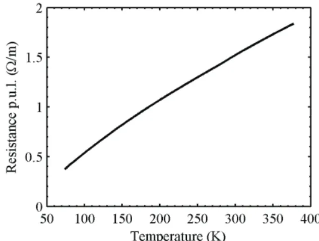
After the evaporation of the LN2 bath, the temperature inside the cryostat slowly rises to reach the ambient temperature. The applied current, the voltage drop and the temperature of the system are acquired at regular time steps. The temperature dependence of the sample electrical resistance 𝑅(𝑇) is therefore measured and is shown in Fig. 1.
2.2. Experimental measurements setup
The measurements are taken while applying a current pulse through the coated conductors at different amplitudes. The durations of the pulses vary between a few tens of milliseconds and 3 seconds. In order to measure the electrical resistance of the sample at any time, a sinusoidal modulation has been added to the current pulse. In particular, the modulation enables us to monitor the resistance value even after the end of the pulse.
Additionally, this prevents offsets on the measured values since the resistance is computed using the ratio of the RMS amplitudes instead of direct values. The modulation signal is a sinusoidal waveform of frequency 3 kHz and with an amplitude of 0.4 A.
The temperature of the sample is calculated using the characterization shown in Fig. 1. Therefore, the temperature is not directly measured during the experiment but the sample itself is used as a sensor to get the temperature value.
Generated voltage signals are transmitted to a voltage-to-current converter configured to reach up to 40 A.
The converter is powered by adjustable voltages between
±12 V and ±24 V. The current pulse was gradually increased from 7 A up to 28 A. The applied current and
Fig. 1. The sample electrical resistance per unit of length as a function of temperature.
Fig. 2. Schematics of the experimental measurement setup.
Fig. 3. Experimental measurements setup. A bare tape is mounted in a 4 wires setup. In front of it, a sample insulated with layers of Kapton® applied directly on the silver surface.
voltage are digitized at a sampling rate of 500 kSa/s and a dynamic of 18 bits. A schematic of the circuit is shown in Fig. 2.
As shown in Fig. 3, the sample is mounted in a 4 wires setup. The current contacts are ensured with Indium conduction sheets. The distance between the voltage taps is 100 mm while the distance between the current leads is 140 mm. The voltage taps are far enough from the current leads to reduce the influence of the heat conduction on the measured section. The sample is immersed in an open LN2
bath at 77 K. An example of measured applied current 11
Heat transfer monitoring between quenched high-temperature superconducting coated conductors and liquid nitrogen
Fig. 4. Example of measured current and voltage obtained with a bare sample. The current pulse has an amplitude of 20 A. The inset shows the 3 kHz modulation.
pulse and voltage is shown in Fig. 4.
The first treatment on measured data consists of extracting their DC and RMS components at 3 kHz. The resistivity of the sample is then determined using the modulation signal as the ratio of the RMS amplitudes of the voltage over the current. This value is averaged on n cycles. The value n = 2 has been used generally in this experiment. This corresponds to a time resolution of 6.6 ms for temperature and power measurements. The power generated inside the tape is calculated using DC components of current and voltage values. In order to avoid damaging the sample, a threshold in the voltage measurement is used to interrupt the current pulse, this insures no overheating of the sample whichever the measuring parameters.
All the measurements were made using a bare tape and three different Kapton® insulating layers (25 µm, 50 µm and 100 µm).
3. RESULTS AND DISCUSSION 3.1. Comparison between adiabatic and real conditions
A common approach to estimate the temperature profile of a HTS-CC in fault condition is to neglect the heat exchange between HTS-CC and LN2 (adiabatic conditions). Under these simplifications, the temperature profile of a HTS-CC can be calculated through numerical models by solving the following heat balance at each time step:
�𝑡𝑘+1�𝑉𝑒𝑥𝑝 ∙ 𝑖𝑒𝑥𝑝�𝑑𝑡 =
𝑡𝑘 �𝑇𝑘+1𝐶𝑝𝐻𝑇𝑆(𝑇)𝑑𝑇
𝑇𝑘
The specific heat, 𝐶𝑝𝐻𝑇𝑆(𝑇) , takes into account the temperature dependence of the substrate and silver stabilizer. The specific heat of the superconducting material is considered constant.
Fig. 5 shows the difference between the temperature computed by the adiabatic model and the temperature measured during the experiment.
Fig. 5. Comparison between the temperature computed by the adiabatic model and the temperature measured during the experiment.
In real RSFCL applications, the fault current is usually assumed to be high and therefore above the critical threshold of the tape. In this case, the heat transfer to LN2
is negligible; hence Texp will tend to the adiabatic case.
However, the most dangerous situation is when the fault current through HTS-CCs is around their 𝐼𝑐 [2]. In this situation and in recovery under load conditions [5], the HTS-CCs are prone to high risk of thermal runaway. In this context, a more effective heat transfer to the LN2 bath could help improving the thermal stability of HTS-CCs subjected to low fault currents.
3.2. Cooling power of the liquid nitrogen bath
Since the resistance is known at each time step of the experiment, the temperature can be deduced using the previously measured resistance-temperature curve 𝑅(𝑇).
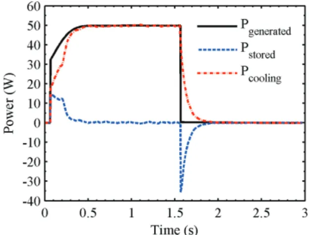
Using this fact, it is possible to evaluate the power corresponding to the energy stored inside the tape during the pulse. Fig. 6 shows the power dissipated inside the tape and the power corresponding to the energy stored in the tape itself; the difference between them being the power exchanged to the bath according to the following equation:
Fig. 6. Generated power, power corresponding to the stored energy and cooling power between the voltage taps (100 mm).
12
Thomas Rubeli, Daniele Colangelo, Bertrand Dutoit, and Michal Vojenčiak
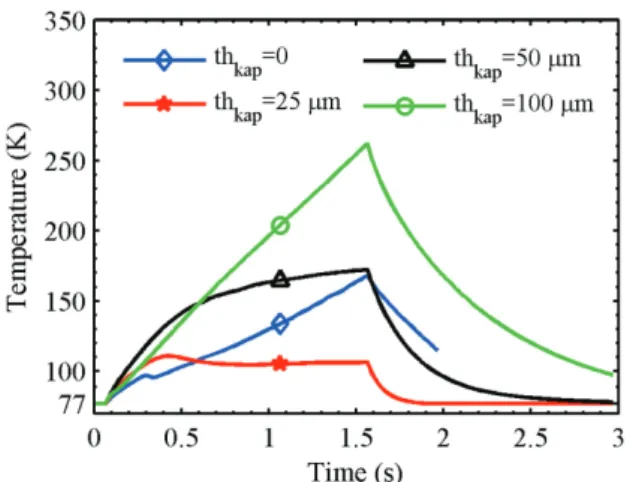
Fig. 7. Temperature reached by the sample for different insulation layers. For the considered cases, the amplitude of the applied current is 20 A.
�𝑡𝑘+1�𝑉𝑒𝑥𝑝 ∙ 𝑖𝑒𝑥𝑝�𝑑𝑡 =
𝑡𝑘 �𝑇𝑘+1𝐶𝑝𝐻𝑇𝑆(𝑇)𝑑𝑇
𝑇𝑘 + 𝑞
The 3 terms of this equation are the generated power (Pgenerated), the power corresponding to the stored energy (Pstored), and the cooling power (Pcooling). Using this scheme, heat fluxes can be evaluated during the pulse as well as during the recooling process.
2.3. Thermal Insulation
As shown in other studies [6], layers of polyimide film, such as Kapton®, have a significant impact on the cooling process of the HTS-CC. The measurements have been performed enclosing the conductor with one or several Kapton® layers. The impact of the insulation is shown in Fig. 7. The different heat exchange regimes are easily identifiable in each of the curves.
For identical current pulses, the different insulation layers have a very different impact on the cooling process. As shown in Fig. 7, for a pulse of 20 A, the bare tape exhibits an unstable state with a continuous temperature increase.
The tape with 25 µm insulation, with the same current pulse, stabilizes itself around 100 K. The tape with 50 µm insulation tends to stabilize itself at a higher temperature.
Finally the tape with 100 µm insulation is again unstable.
We can conclude that for these experimental conditions an insulated tape with a thickness between 25 and 50 µm is much more stable than either a bare or a highly insulated tape.
3.3. Recovery speed
In this last step we have been able to determine a time constant characterizing the recooling process. This is done by fitting the tails of the curves with an exponential decay law. These fits can be seen on Fig. 8 for each different cooling condition. The same observations as above are true for the recooling speed, as shown in the table below the fastest recooling time is obtained with 25 µm insulation.
Fig. 8. Temperature profile of the sample during the recooling process. The exponential decay time (τ) is shown in the figure.
TABLEI EXPONENTIAL DECAY TIME.
Bare 25 𝝁𝒎 50 𝝁𝒎 100 𝝁𝒎
𝝉 0.49 s 0.09 s 0.28 s 0.66 s
4. CONCLUSION
This paper proposed a technique to precisely measure in real time the temperature and the heat exchanged to the bath of a quenched RSFCL tape immersed in liquid nitrogen. The comparison with an adiabatic model shows that the cooling power has to be taken into account when designing and dimensioning HTS-CC for RSFCL application. This aspect is particularly important to obtain the best stabilization of a HTS-CC, which is always more or less inhomogeneous. For optimal stabilization, a thermal insulation with a thickness adapted to the operating conditions has to be used.
REFERENCES
[1] M. Noe et al., “Conceptual Design of a 24 kV, 1 kA Resistive Superconducting Fault Current Limiter,” IEEE Trans. Appl.
Supercond., vol. 22, no. 3, 5600304, 2012.
[2] D. Colangelo and B. Dutoit, “Inhomogeneity Effects in HTS Coated Conductors Used as Resistive FCLs in Medium Voltage Grids,”
Supercond. Sci. Tech., vol. 25, 095005, 2012.
[3] V. K. Dhir, “Boiling heat transfer,” Annu. Rev. Fluid Mech., vol. 30:
365-401, 1998.
[4] SuperPower Inc., http://www.superpower-inc.com/
[5] A. Berger, M. Noe and A. Kudymow, “Recovery characteristic of coated conductors for superconducting fault current limiters,” IEEE Trans. Appl. Supercond., vol. 21, no. 3, p.1315-1318, 0501605, 2011.
[6] S. Hellmann and M. Noe, “Influence of different surface treatments on the heat flux from solids to liquid nitrogen,” IEEE Trans. Appl.
Supercond., vol. 24, no. 3, 0501605, 2014.
13