Parametric Analysis of the Solar Radiation Pressure Model for Precision GPS Orbit Determination

1. Introduction

The POD (Precise Orbit Determination) of satellites including GPS (Global Positioning System) is generally conducted by the dynamic approach using force models.

The dynamic orbit determination is, in principle, an initial value problem of the ordinary differential equation. The primary parameters in the dynamic POD are the so-called the initial conditions, that is, having position and velocity at the initial epoch of integration in the inertial frame. The

initial epoch is not necessarily the earliest time of the arc, but rather any epoch within the arc. This is because the orbit error grows as integration proceeds and, therefore, the middle epoch of the arc can be a suitable candidate for the initial condition. The numerical integrator - specifically, the ODE (Ordinary Differential Equation) solver - would be particularly advantageous if it is bi-directional. In addition to the initial conditions, the most important concern in POD is how we can accurately calculate the SRP (Solar Radiation Pressure).

https://doi.org/10.7848/ksgpc.2017.35.1.55

Parametric Analysis of the Solar Radiation Pressure Model for Precision GPS Orbit Determination

Bae, Tae-Suk

Abstract

The SRP (Solar Radiation Pressure) model has always been an issue in the dynamic GPS (Global Positioning System) orbit determination. The widely used CODE (Center for Orbit Determination in Europe) model and its variants have nine parameters to estimate the solar radiation pressure from the Sun and to absorb the remaining forces. However, these parameters show a very high correlation with each other and, therefore, only several of them are estimated at most of the IGS (International GNSS Service) analysis centers. In this study, we attempted to numerically verify the correlation between the parameters. For this purpose, a bi-directional, multi-step numerical integrator was developed. The correlation between the SRP parameters was analyzed in terms of post-fit residuals of the orbit. The integrated orbit was fitted to the IGS final orbit as external observations. On top of the parametric analysis of the SRP parameters, we also verified the capabilities of orbit prediction at later time epochs. As a secondary criterion for orbit quality, the positional discontinuity of the daily arcs was also analyzed. The resulting post-fit RMSE (Root-Mean-Squared Error) shows a level of 4.8 mm on average and there is no significant difference between block types. Since the once-per-revolution parameters in the Y-axis are highly correlated with those in the B-axis, the periodic terms in the D- and Y-axis are constrained to zero in order to resolve the correlations. The 6-hr predicted orbit based on the previous day yields about 3 cm or less compared to the IGS final orbit for a week, and reaches up to 6 cm for 24 hours (except for one day). The mean positional discontinuity at the boundary of two 1-day arcs is on the level of 1.4 cm for all non-eclipsing satellites.

The developed orbit integrator shows a high performance in statistics of RMSE and positional discontinuity, as well as the separations of the dynamic parameters. In further research, additional verification of the reference frame for the estimated orbit using SLR is necessary to confirm the consistency of the orbit frames.

Keywords : GPS, Orbit, Solar Radiation Pressure, Numerical Integrator

Original article

Received 2017. 01. 10, Revised 2017. 02. 02, Accepted 2017. 02. 09

1) Member, Dept. Geoinformation Engineering, Sejong University (E-mail: [email protected])

This is an Open Access article distributed under the terms of the Creative Commons Attribution Non-Commercial License (http://

In this study, we developed a numerical integrator to generate a GPS orbit based on a dynamic model. It calculates the forces acting on the satellite and integrates them numerically to obtain the position and velocity of the satellite at other time epochs (Bae, 2006; Bae et al., 2007). Among many force components, the SRP modeling is the most significant and complicated process in the GPS orbit calculation. Most dynamic force modeling follows the IERS Conventions (2010) (Petit and Luzum, 2010) and some minor effects, such as Earth albedo and others, are also considered. However, due to the correlation between the SRP parameters, most analysis centers estimate only a few of them. As can be seen in Table 1, seven out of nine analysis centers participating in the combination of the IGS final orbit product use the CODE solar radiation pressure (denoted as RPR) model or its variants, though the estimated parameters are slightly different. Therefore, it can be supposed that the IGS final orbit is much closely related to the CODE RPR model than others.

In this paper, the concept of numerical integration for the satellite orbit determination is first described in Section 2. Since numerical integration is performed in the inertial frame, wherein Newton’s law of motion holds, the transformation between the terrestrial and inertial frames is necessary. Three different transformation methods are considered in this study. We thoroughly analyzed the correlations between the estimated SRP parameters in the numerical sense. The GPS orbit was processed over the

course of a week in 2009 (GPS week 1540, day of year 193- 199). The performance of the orbit integrator was evaluated in terms of orbit fit with respect to the IGS final orbit and the orbit prediction based on the estimated parameters. The positional differences at the boundary of the daily arcs were also verified for all satellites.

2. Orbit Integration

As mentioned above, the dynamic orbit determination can be represented by the second-order ODE in the extended state vector (se Eq. (1)) (Montenbruck and Gill, 2005):

(1)

where r r are the position and velocity vectors, respect- , ively, and r , the acceleration of the satellite, is a function of them. Since it is difficult to calculate the forces acting on the satellites due to both the irregular shape and the complex characteristics of the surface of the body, a numerical method to integrate the differential equation is recommended for highly accurate orbit solutions. A number of ODE solvers have been successfully applied in the satellite orbit determination.

Since calculating the acceleration for the satellite requires intensive arithmetic operations, it may be preferable to use multi-step methods that store past data points from previous steps to reduce the total number of function evaluations

( , , ) dt

   

   

   

r r

r  a r r 

Table 1. SRP models and parameter estimation for the GPS final orbit used in the IGS analysis centers (http://igscb.jpl.nasa.gov/igscb/center/analysis/)

AC SRP model SRP parameters to estimate

CODE CODE RPR Constants in D, Y and X, periodic terms in X

EMR GSPM_EPS Y bias and scale in D, stochastic Y bias and X/Z solar scale

ESA CODE RPR Constants in D, Y and B, periodic terms in B

GFZ CODE RPR Constants in D, Y and X, periodic terms in X

GRG CODE RPR Y bias, periodic terms in X and D

JPL GSPM-10 Y bias, constants in X and Z

MIT CODE RPR Constants in D, Y and B, periodic terms

NOAA CODE RPR Constants in D, Y and B, periodic terms in B

SIO CODE RPR Constants in D, Y and B, periodic terms in each direction (total 9 parameters)

(Beutler, 2005; Montenbruck and Gill, 2005).

In general, SRP acting on a satellite is relevant to the geometric configuration with respect to the Sun. As described in Section 1, many SRP models have been applied for the dynamic orbit determination of GPS satellites. For instance, Beutler et al. (1994) proposed the ECOM, which is composed of the direct terms and once-per-revolution parameters in three orthogonal axes (see Eq. (2)) (Springer et al., 1999a, 1999b).

(2)

with e 

: unit vector satellite-Sun, positive towards the Sun e 

: unit vector along the spacecraft solar-panel axis e 

: unit vector defined by e 

= e e 

× 

^u : argument of latitude of the satellite,

and the subscripts C and S in D, Y, and B terms represent the cosine and sine terms, respectively. The periodic terms in Eq. (2) can absorb the remaining unmodeled forces. Since the GPS satellites experience eclipsing by the Earth in a certain condition (and sometimes also by the Moon), the partial SRP should be applied according to the area of the Sun as seen from the satellite. The conical model for the Earth’s shadow is used in this study (Montenbruck and Gill, 2005).

The position and the velocity at a certain epoch are used as the ICs (Initial Conditions) in the dynamic orbit determination. These ICs, given in the middle of the arc in this study, are propagated throughout the arc using the developed bi-directional, multi-step integrator. Alongside with the position and the velocity, the partial derivatives of the acceleration with respect to the ICs are integrated together. The partial derivatives are used to estimate the parameters based on the external information, for example, the GPS range measurements or the pseudo-observations as the published final orbit.

One aspect to be mentioned here is that all numerical integration should be performed in the inertial frame. The coordinates of the GPS reference stations, as well as the

IGS final orbit in SP3 format, are given in the terrestrial frame. Therefore, the transformation between terrestrial and celestial frames should be considered, because GPS orbit integration requires a considerably large number of transformations. Three approaches were suggested by McCarthy and Petit (2003), classified by the non-rotation origin and the nutation model. That is, Method 1 refers to IAU 1976 precession and 1980 nutation model; Method 2 to IAU2000A with CIO (Celestial Intermediate Origin); and, finally, Method 3 to IAU2000A with the classical approach.

Method 1 requires the minimum computation time with about 0.05 mas of rotation angle difference, which is within a permissible range. Methods 2 and 3, which use the same model for precession and nutation, show a comparable performance in terms of accuracy (Bae, 2009).

3. Analysis of Correlations and Orbit Accuracy

The GPS satellite orbit was integrated for a week (GPS week 1540) using the developed orbit integrator. The solar radiation pressure model of ECOM (Extended CODE Orbit Model) was primarily tested in this study. During the period of the testing week, PRN 1 was estimated with unknown satellite clock information, resulting in an unstable satellite condition. Therefore, to remove the unexpected outliers, this satellite was excluded from the analysis. Other than that, no satellite problems were reported during this period (http://

www.navcen.uscg.gov). The propagated orbit was fitted to the IGS final orbit to estimate the orbit parameters in the inertial frame. A total of 15 parameters were estimated including six initial conditions (position and velocity) and nine solar radiation parameters in three orthogonal directions as described in Eq. (2). The overall post-fit residuals were calculated based on the following equation (see Eq. (3)):

(3)

where e is the residuals of the orbit after least-squares adjustment, N is the number of satellites to be integrated, and n

represents the total number of observations in the calcu- lation.

1

1

rms e e

n

= ∑ ^{ }

0 0 0

( cos sin )

( cos sin ) ( cos sin )

RPR D Y B

C S D

C S Y

C S B

a D e Y e B e

D u D u e

Y u Y u e

B u B u e

= + +

+ +

+ +

+ +

   







Table 2 shows the strategy used for GPS orbit integration.

To reduce the edge effect, the integration was performed for 32 hours, that is, one full day (24 hours) plus 4 more hours on each side in order. The initial condition of the satellite is given at the center of the arc, which is noon of the integration day. Therefore, numerical integration was performed in both directions: first backward and then forward integration. The initial condition of position and velocity can be obtained in many ways, either from the results of the previous day or the rapid orbit. The initial values for the SRP parameters were all set to zeroes, except for the direct force component, which is given by the a priori ROCK model (Fliegel et al., 1992). The propagated orbit from the initial condition into both sides (96 epochs for 24 hours, 0:00-23:45) was fitted to the IGS final orbit as pseudo-observations. The fitting process was done by the least-squares adjustment: namely, the design matrix was obtained by the propagated variational partials, that is, the partial derivatives of the acceleration with respect to the parameters. The difference between pseudo-observation and the propagated orbit served as an observation to estimate the corrections to the initial value of each parameter.

The post-fit RMSE (Root-Mean-Squared Error) for one week of GPS satellite orbit is about 4.8 mm on average. Fig.

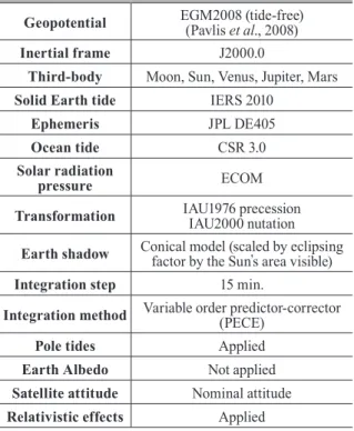
1 shows the average correlation coefficients in an absolute sense for all satellites after estimating nine SRP parameters on DOY 195. As can be seen in Fig. 1, the constant term (D0 in Eq. (2)) in the Sun-satellite direction plays an important role and, therefore, it is correlated with most parameters. It should be noted that the once-per-revolution parameters in the Y- and B-axis are highly correlated, that is, the cosine term in the Y-axis (Yc) vs. the sine term in the B-axis (Bs), and vice versa (Ys vs. Bc). This phenomenon is commonly seen in almost all satellites (see Fig. 2). Another significant correlation is related to the constant term in the B-axis (B0), which is correlated with the periodic terms in the D-axis (Dc and Ds are also highly correlated with each other).

Fig. 2. Correlation coefficients (absolute values) between Ys and Bc (DOY 195) Geopotential EGM2008 (tide-free)

(Pavlis et al., 2008)

Inertial frame J2000.0

Third-body Moon, Sun, Venus, Jupiter, Mars

Solid Earth tide IERS 2010

Ephemeris JPL DE405

Ocean tide CSR 3.0

Solar radiation

pressure ECOM

Transformation IAU1976 precession IAU2000 nutation Earth shadow Conical model (scaled by eclipsing

factor by the Sun’s area visible)

Integration step 15 min.

Integration method Variable order predictor-corrector (PECE)

Pole tides Applied

Earth Albedo Not applied

Satellite attitude Nominal attitude Relativistic effects Applied

Table 2. Summary of the strategy for orbit integration

Fig. 1. Average correlation coefficients (absolute values) between parameters (DOY 195).

Diagonal terms are excluded

In order to check the contribution of each parameter to the post-fit residuals, the RMSE was calculated using the adjusted observations (see Eq. (4)):

k k k

ˆ

v  = A ξ (4) where A

and ξ ^ˆ

correspond to the variational partials and the estimates of parameter k, respectively.

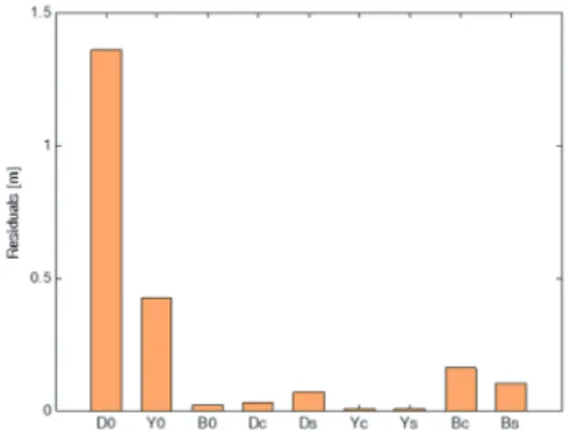
Fig. 3 shows the contribution of each parameter in terms of RMSE. As can be expected, the constant term in direct Sun-satellite direction takes the most dominant portion on the adjusted observation, followed by Y0. The periodic terms in the B-axis also make significant contributions to the adjusted

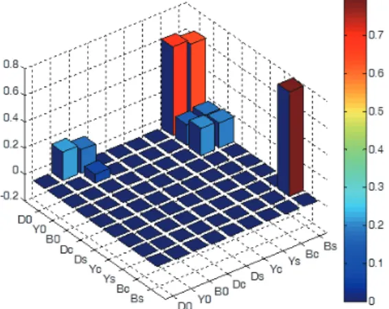
observation, which are highly correlated with the periodic terms in the Y-direction. As can be seen in Fig. 4, the term in the B-axis has an order of magnitude larger than that in the Y-axis and these two parameters are highly correlated in terms of the adjusted observations as calculated by Eq. (4).

The contribution to the adjusted observations shows a periodic behavior that is close to the orbital period of GPS satellites.

Due to the complex, high correlation between the parameters, reducing these correlations between parameters was considered. The idea is that the constant terms in each direction are preferentially estimated for the orthogonality of the parameters, though the contribution of B0 to the residuals is somewhat small (see Fig. 3). Since the constant term in the B-axis is to be estimated, the highly correlated parameters Dc and Ds should be suppressed in the estimation process. In addition, two periodic terms in the Y-axis are also correlated with those in the B axis; therefore, it was decided not to estimate Yc and Ys.

Based the aforementioned reasons, the least-squares adjustment with fixed constraints was adopted to estimate the reduced orbital parameters that regulate the correlations between parameters. The Gauss-Markov model with fixed constraints was applied as follows (see Eq. (5)):

2 1

1 1 1 0

0

~ (0, )

,

n n m m n

l m

T T

y A e e P

K

rkK l rk A K m

ξ σ

κ ξ

× × × × −

×

= + Σ =

=

 

=   =

(5)

where P ^and σ

correspond to the weight matrix and the unitless variance component, respectively. The (residual) observation vector y represents the difference between the external orbit and the propagated one; the design matrix A can be obtained by numerically integrating the variational partials. The unknown parameter ξ is common to both the observation equation (top) and the fixed constraints (bottom) in Eq. (5). The normal equation for the LESS (LEast-Squares Solution) can be expressed by Eq. (6) (Snow, 2002).

0

ˆ 0 ˆ

T

c

N K K

ξ λ κ

     

  =

   

   

   

(6) Fig. 3. Overall contributions of parameters on the

residuals (DOY 195)

Fig. 4. Contributions of parameters on the adjusted

observations (PRN 30 on DOY 195)

Note: Yc refers to the left axis and Bs to the right axis

where λ is the Lagrangian multiplier and [ ^{N c} ] ^{= A P A y}

[ ] [ ^{N c} ] ^{= A P A y}

[ ] . The variance component is given by

2

0

ˆ

ˆ e Pe

with e y A n m l

σ = = − ξ

− +

 

 (7)

Once the fixed constraints were applied, as expected, the correlations between parameters considerably reduced (see Fig. 5). In addition, the dispersion also decreased, not only for the constrained parameters, but for all estimated parameters.

For the purpose of verifying the quality of the estimated orbit, two tests were performed: 1) orbit prediction based on the estimated parameters from the previous day, up to 24 hours; and 2) orbit discontinuity between two consecutive 1-day arcs. Figs. 6 and 7 show an orbit prediction for 6 hours and the accumulated statistics up to 24 hours, respectively, for a total of 30 satellites. Once the initial conditions as well as the dynamic SRP parameters were estimated, this orbit was predicted for the next day and compared with the IGS final orbit. As can be seen in Fig. 6, except for DOY 194, the 6-hr prediction has an accuracy of better than 3 cm for the whole week. If the predicted arc is extended up to 24 hours, the accumulated post-fit RMSE is gently increasing up to 4 cm for the arc of about 15 hours and additional increases continue as the arc gets longer (see Fig. 7).

As a final check for orbit quality, the PD (Positional Discontinuity) of the orbit was tested for arcs of two consecutive days. Griffiths and Ray (2009) suggested the PD as an alternative criterion to IGS orbit accuracy estimates.

The PD represents the magnitude of the 1-D shift in the satellite orbit at the boundary of two consecutive 1-day arcs (A and B), which is defined by Eq. (8).

3

B A B A B A

X X Y Y Z Z

PD − + − + −

= (8)

With a slightly different boundary from the approach by Griffiths and Ray (2009), the discontinuity was evaluated at midnight by extending one epoch for the solution of the previous day. Fig. 8 shows the PD of each satellite, excluding Fig. 5. Same as Fig. 1, except for the fixed constraints

Fig. 6. The 6-hr orbit prediction for GPS Week 1540

Fig. 7. Orbit prediction results for 24 hours (GPS week 1540).

Each data point represents the orbit prediction results up to

the hour corresponding to the axis of abscissa

4 satellites in eclipse, for each arc pair alongside with the mean PD values for all satellites. The mean PD is less than 1.4 cm for the whole week, reaching the maximum value of about 3.4cm. Even when the eclipsing satellites are considered, the mean PD is about 1.46 cm on average and 4.35 cm at the maximum.

4. Discussion and Conclusions

In this study, dynamic method, the most common approach to satellite orbit determination, was applied. The post-fit residuals analyzed over the course of a week show that there is no significant difference between Block types in terms of RMSE. The statistical results for eclipsing satellites are slightly worse, but do not show any unusual behavior.

The CODE RPR model with its variants is commonly used as the SRP model in the GPS orbit determination. A total of nine parameters cover the bias terms, as well as the once-per- revolution components in three orthogonal directions. The bias term in the Sun-satellite direction is highly correlated with other parameters, especially, the periodic parameters in the Y- and B-axis. The most significant correlation can be found in the parameters between the Y- and B-axis, which is nearly coincident in frequency. Since the bias terms occupy most of the residuals, these three terms have priority in the estimation. Other than the bias terms, two periodic terms, Bc and Bs, contribute the most to the residuals; these are thus determined for the estimation of dynamic parameters

in order to resolve the correlation between parameters.

The remaining four parameters are suppressed by the fixed constraints, which set the parameters (corrections) to zero.

With this process, the parameters can mostly be separated from each other, resulting in improved uncertainties for the estimated parameters. However, the overall dispersion of the residuals is slightly larger than in the unconstrained case.

The residuals that correspond to the constrained parameter are absorbed by the associated parameters.

For the verification of the estimated orbit quality, an accumulated accuracy of the predicted orbit was calculated by comparing it with the IGS final orbit. The prediction accuracy was found to be modestly increasing up to 6 cm, except for DOY 199, showing a very similar pattern for the entire week. On the other hand, the positional discontinuity at the boundary of two 1-day arcs shows a good agreement, although the two arcs used different initial conditions (24 hours apart).

No significant decline in the orbit accuracy for the eclipsing satellites was observed; however, these should be tested further in future research, because the attitude during the eclipse period can affect a one-way range for Block IIA satellites, resulting in errors for positioning, for example, PPP (Precise Point Positioning). The relationship between the SRP models and the GPS orbit scale should also be tested in a time series.

Acknowledgments

This research was supported by a grant(16RDRP-B076564 03) from Regional Development Research Program funded by Ministry of Land, Infrastructure and Transport of Korean government.

References

Bae, T.S. (2006), Near Real-Time Precise Orbit Determination of Low Earth Orbit Satellites using an Optimal GPS Triple- Differencing Technique, Report No. 481, Department of Civil and Environmental Engineering and Geodetic Science, The Ohio State University, Columbus, Ohio, 121p.

Bae, T.-S., Grejner-Brzezinska, D., and Kwon, J. (2007), Fig. 8. Positional discontinuity at midnight for all non-

eclipsing satellites (GPS week 1540)

Efficient LEO dynamic orbit determination with triple differenced GPS carrier phases, The Journal of Navigation, Vol. 60, No. 2, pp. 217-232.

Bae, T.S. (2009), A preliminary study of near real-time precision satellite orbit determination, Journal of Geomatics, Vol. 27, No. 1, pp. 49-56.

Beutler, G., Brockmann, E., Gurtner, W., Hugentobler, U., Mervart, L., Rothacher, M., and Verdun, A. (1994), Extended orbit modeling techniques at the CODE processing center of the international GPS service for geodynamics (IGS): theory and initial results, Manuscripta Geodaetica, Vol. 19, pp. 367-386.

Beutler, G. (2005), Methods of Celestial Mechanics, Springer- Verlag, Berlin Heidelberg.

Fliegel, H.F., Gallini, T.E., and Swift, E.R. (1992), Global positioning system radiation force model for geodetic applications, Journal of Geophysical Research, Vol. 97, No. B1, pp. 559-568.

Griffiths, J. and Ray, J.R. (2009), On the precision and accuracy of IGS orbits, Journal of Geodesy, Vol. 83, No.

3, pp. 277-287.

McCarthy, D.D. and Petit, G. (2003), IERS Technical Note 32, IERS Conventions (2003), IERS Conventions Centre, Verlag des Bundesamts für Kartographie und Geodäsie, Frankfurt am Main.

Montenbruck, O. and Gill, E. (2005), Satellite Orbits:

Models, Methods, And Applications, Springer-Verlag, Berlin Heidelberg New York.

Pavlis, N.K., Holmes, S.A., Kenyon, S.C., and Factor, J.K.

(2008), An Earth gravitational model to degree 2160:

EGM2008, EGM General Assembly 2008, Vienna, Austria.

Petit, G. and Luzum, B. (2010), IERS Technical Note 36, IERS Conventions (2010), IERS Conventions Centre, Verlag des Bundesamts für Kartographie und Geodäsie, Frankfurt am Main.

Snow, K. (2002), Applications of Parameter Estimation and Hypothesis Testing to GPS Network Adjustment, Report No. 465, Department of Civil and Environmental Engineering and Geodetic Science, The Ohio State University, Columbus, Ohio, 107p.

Springer, T.A., Beutler, G., and Rothacher, M. (1999a),

Improving the orbit estimates of GPS satellites, Journal of Geodesy, Vol. 73, No. 3, pp. 147-157.

Springer, T.A., Beutler, G., and Rothacher, M. (1999b), A

new solar radiation pressure model for GPS satellites. GPS

Solutions, Vol. 2, No. 3, pp. 50-62.