Accuracy Evaluation of DEM generated from Satellite Images Using Automated Geo-positioning Approach

1. Introduction

Geo-positioning of high resolution satellite image is the most important pre-processing step. Geo- positioning is involved in the process of establishing a geometric relationship between image space and object space, and thus enables image coordinates to transform

ground coordinates in a map projection. In this step, there are two central requirements -speed and accuracy.

So far, a number of researchers have made an effort to improve geo-positing accuracy, but most of them include a human element. These days, however, we are retrieving huge amounts of satellite image data, and these data should be processed as soon as possible.

Accuracy Evaluation of DEM generated from Satellite Images Using Automated Geo-positioning Approach

Kwan-Young Oh*

**, Hyung-Sup Jung* and Moung-Jin Lee**

*Department of Geoinformatics, The University of Seoul

**Environmental Assessment Group/Center for Environmental Assessment Monitoring, Korea Environment Institute

Abstract : S The need for an automated geo-positioning approach for near real-time results and to boost cost-effectiveness has become increasingly urgent. Following this trend, a new approach to automatically compensate for the bias of the rational function model (RFM) was proposed. The core idea of this approach is to remove the bias of RFM only using tie points, which are corrected by matching with the digital elevation model (DEM) without any additional ground control points (GCPs). However, there has to be a additional evaluation according to the quality of DEM because DEM is used as a core element in this approach. To address this issue, this paper compared the quality effects of DEM in the conduct of the this approach using the Shuttle Radar Topographic Mission (SRTM) DEM with the spatial resolution of 90m. and the National Geographic Information Institute (NGII) DEM with the spatial resolution of 5m. One KOMPSAT-2 stereo-pair image acquired at Busan, Korea was used as experimental data. The accuracy was compared to 29 check points acquired by GPS surveying. After bias-compensation using the two DEMs, the Root Mean Square (RMS) errors were less than 6 m in all coordinate components. When SRTM DEM was used, the RMSE vector was about 11.2m. On the other hand, when NGII DEM was used, the RMSE vector was about 7.8 m. The experimental results showed that automated geo-positioning approach can be accomplished more effectively by using NGII DEM with higher resolution than SRTM DEM.

Key Words : Automated geo-positioning, KOMPSAT, SRTM DEM, NGII DEM http://dx.doi.org/10.7780/kjrs.2017.33.1.7

Received February 10, 2017; Revised February 15, 2017; Accepted February 20, 2017.

†

Corresponding Author: Moung-Jin Lee ([email protected])

This is an Open-Access article distributed under the terms of the Creative Commons Attribution Non-Commercial License (http://creativecommons. org/licenses/by-nc/3.0) which permits unrestricted non-commercial use, distribution, and reproduction in any medium, provided the original work is properly cited

ISSN 2287-9307 (Online)

Article

What is more, the number of earth observing satellites is expected to continue growing (Euroconsult, 2010).

This is the reason why speed is a crucial factor in the geo-positioning step. Not surprisingly, the need for an automated geo-positioning process to achieve near real- time results and boost cost-effectiveness has become increasingly urgent in recent times. In general, the rational function model (RFM) is preferred to explain the geometric relationship for high-resolution satellite images. This is a common mathematic model, which is constructed with rational polynomial coefficients (RPCs). These RPCs are computed by each satellite system based on orbital position and orientation and a rigorous physical sensor model. However , RFM constructed from RPCs alone do not meet accuracy requirements. That is because RPCs cause inevitable errors from the uncertainty of GPS receivers, star sensors and gyroscopes. For example, RPCs accuracy of KOMPSAT-2 (the Korea Multi-Purpose Satellite- 2) is about 80 m (90%) in the horizontal direction (Seo, et al., 2008). This accuracy is definitely not sufficient with regard to geospatial information production. Of course, many methods have been proposed to solve this problem. All of these methods are referred to as the bias-compensation method. The bias-compensation method generally needs precise ground control points (GCPs), which include ground coordinates and their corresponding image points (Fraser et. al., 2006). GCPs can be obtained from GPS-survey or precise reference data. The most common way to collect GCPs is to use GPS-survey. This is the certain way to get the best performance, but is time-consuming and laborious.

Moreover, this kind of field-survey is not feasible in remote and inaccessible areas (Oh and Lee, 2014).

Accordingly, many researchers have begun to make an effort to reduce the necessity of GCPs and to increase cost-effectiveness by automating the entire process (Inglada and Giros, 2004). Among others, some remarkable studies have attempted to only use the shuttle radar topographic mission (SRTM) DEM,

without GCPs collecting. SRTM DEM is near-global elevation - freely available online, with spatial resolution of 90 m. Goncalves (2006) carried out the correlation matching between a relative DEM derived from SPOT stereo-image and SRTM DEM, resulting in an accuracy that is about 10 m. Ataseven and Alatan (2010) has considered the matter from another view point - SRTM DEM is projected in IKONOS images space - to improve geo-positioning accuracy. This, however, has a limit for massive satellite images, requiring rapid updating and refinement. That is why relative DEM generation is a very arduous, time-consuming process.

Therefore, Oh and Jung (2016) proposed a new approach to overcome this limitation. To begin with, this approach does not need relative DEM generation.

Instead, tie points derived from stereo-image randomly are needed. Next, another step is finding the maximum correlation position by matching tie points to DEM, resulting in refined tie points. Finally, these refined tie points enable the establishment of the corrected RFM.

In experiment results, the accuracy calculated by check

point was within 9 m in X-, Y-, Z-direction

respectively. However, a few systematic errors still

remain in the portions of the image area after this kind

of proposed processing. This is why Oh and Jung

(2016)’s approach supposes that the errors of all tie

points are the same. These results indicate that partial

adjustment may be needed depending on different

positions in the image area. However, if SRTM DEM

is used as reference data, it may not work, on account

of the limited accuracy in SRTM DEM. In the

approach proposed in this study, accuracy according

to DEM quality was compared and analyzed using

high resolution National Geographic Information

Institute (NGII) DEM. Experiments were carried out

for a KOMPSAT-2 stereo-pair image. The accuracy of

the proposed approach was compared to check-points

acquired by GPS survey.

2. Study Area and Test Data 1) Study Area and KOMPSAT-2 Stereo-Pair

Image

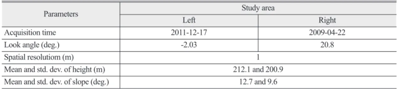
In this paper, we used one KOMPSAT-2 stereo-pair image acquired at Busan, Korea, which is located in the Korea (Fig 1). It contained plains, lakes, mountains and man-made structures such as buildings, roads, and bridges. The stereo-pair image consisted of a left image with -2.0˚ look angle and a right image with 20.8˚ look angle and were acquired on 17 December 2011 and 22 April 2009 respectively. The study area has some height variations. It has average and standard deviation of height at 212.1 m and 200.9 m respectively (Table 1). Furthermore, the study area includes some slope variations. The mean and root mean square deviation

of terrain slope were about 12.7 and 9.6 deg., respectively. It is notable that these topographic features would have an influence on the accuracy of the proposed approach. This is because the Oh and Jung (2016)’s approach does not work if the study area is perfectly flat. This constraint stands out well in the study area. In other words, the study area is suitable for carrying out this research.

2) SRTM DEM and NGII DEM

The DEMs acquired for this research were 90 m spatial resolution SRTM DEM and 5 m spatial resolution NGII DEM. Oh and Jung (2016) carried out the accuracy experiment only using SRTM DEM. On the other hand, if a high-resolution DEM is used rather than SRTM DEM, the accuracy of the Table 1. Characteristics of KOMPSAT-2 stereo image pair used for this study

Parameters Study area

Left Right

Acquisition time 2011-12-17 2009-04-22

Look angle (deg.) -2.03 20.8

Spatial resolutiom (m) 1

Mean and std. dev. of height (m) 212.1 and 200.9

Mean and std. dev. of slope (deg.) 12.7 and 9.6

Fig. 1. KOMPSAT-2 stereo pair used in this study: (a) Left image, (b) Right image.

(a) (b)

Oh and Jung (2016)’s approach could be expected to improve. For this reason, we conducted a comparative experiment using 5m NGII DEM provided by the National Geographic Information Institute (NGII). In 2014, NGII tested the height accuracy of SRTM DEM and NGII DEM for all South Korea (Table 2). For NGII DEM, the maximum and minimum height error were - 23.6 m and 0 m, respectively. The mean, standard deviation, and RMSE were -0.7 m, 4.8 m, and 4.9 m, respectively. On the other hand, for the SRTM DEM, the maximum and minimum height errors were -21.4 m and 0 m, respectively. Mean, standard deviation, and RMSE were -3.0 m, 4.3 m, and 5.2 m, respectively. The RMSE and standard deviation for both DEMs were less than 5m. The maximum error of NGII DEM was about 2 m higher than SRTM DEM. On the other hand, SRTM DEM is about 4 times higher than NGII DEM in the case of average of error. In other words, it can be

expected that NGII DEM improves accuracy of Oh and Jung (2016)’s approach more than SRTM DEM.

3) Check Points and Tie Points

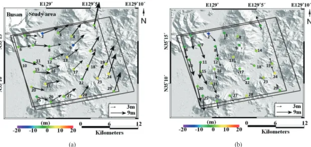
In order to test the performance of the proposed method, 29 check points were examined for the study area. The check points were acquired by GPS field surveys, and were well distributed across the whole scene, and measured at an accuracy of 0.1 m from horizontal to vertical dimensions. Fig. 2 shows the distribution of check points and tie points in the study area. The total of 180 tie points were extracted from stereo-pair image using the image matching method.

The extracted tie points were well distributed, and included height variation.

3. Methodology

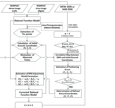
Fig.3 shows the flow chart of the proposed approach.

With conventional image match techniques, tie points are extracted in the stereo-pair. RFM enables the estimatation of the initial ground coordinates of the tie points. Note that these initial ground coordinates include errors in the RPCs . In other words, these tie points are projected to inaccurate ground positions depending on the geometry quality of the RPCs. The next step is to determine those errors across the entire tie points by means of correlation matching with DEM.

After successful refinement of tie points, we can establish the corrected RFM.

1) Extraction of Tie Points

Tie points are geographical features, which are clear in the stereo-pair image. Generally, automatic image

Table 2. Hight Accuracy of SRTM DEM and NGII DEM in the South Korea (Modified from NGII(2014))

Hight error DEM max (m) min (m) mean (m) std. dev.(m) RMSE(m)

SRTM (90m) -21.4 0 -3.0 4.3 5.2

NGII (5m) -23.6 0 -0.7 4.8 4.9

Fig. 2. Distribution of check points and tie points in the study

area. Study area included 29 check points and 180 tie

points. Open and solid diamonds denote the check and

tie points, respectively.

matching techniques are used for finding tie points. In this paper, we used automatic image matching techniques proposed by Wang (1999). The method involves a feature point matching approach based on a pyramid strategy. Since this method uses the sensor model information, it is faster than structural matching.

More details can be found in Leica Geosystems (2004).

2) Calculation of Initial Ground Coordinates The extracted tie points include image coordinates in stereo-pair image but have no ground coordinates.

To estimate ground coordinates, the stereo-pair image to the ground space projection has to be carried out using RFM. Using inverse RFM, the ground coordinates can be estimated. But, these ground coordinates are incorrect because of errors in the RPCs themselves.

3) Refinement of Initial Ground Coordinates Initial ground coordinates of tie points, which are estimated from RFM, have systematic errors. It can be assumed that these errors are absolutely large but relatively small. That is to say, errors of the initial ground coordinates of tie points can be large, but the error differences between adjacent tie points can be small. From this assumption, the initial ground coordinates of tie points can be refined by using correlation matching between the heights of initial ground coordinates and the heights of DEM (Oh and Jung, 2016).

p(n.m) = (1)

Where p is the correlation coefficient, Z

and Z

w

[Z

_ ][Z

(X

+ m∆X, Y

+ n∆Y) _ ]

Np

i =1

∑

Z

Z

w

[Zi_ ] Z

[Z

(X

+ m∆X, Y

+ n∆Y) _ Z

]

Np

i =1

∑

Np

i =1

∑

Fig. 3. Flow chart of the Oh and Jung(2016)’s approach.

are the height of the ground coordinate for i th tie point and the height of DEM corresponding to horizontal ground coordinate (X

and Y

). and are averages of Z

and Z

(•), respectively. ∆X and ∆Y are cell sizes of the correlation coefficient map in X and Y directions. n and m are numbers of lines and pixels for the correlation coefficient map.

4) Estimation of RFM Adjustment Model Parameters

In Oh and Jung(2016)’s approach, the well-known affine transformation is used RFM Adjustment Model.

This polynomial equation is added to image coordinates respectively, resulting in the improved positional information (Oh and Jung, 2016).

4. Results and Analysis

In this research, 29 check points were acquired by GPS surveys, and then used for testing the performance of the proposed approach using SRTM DEM and NGII DEM. Firstly, the three- dimensional geo-positioning using RFM was applied to the stereo-pair image. In study area, the average error calculated was 14.3 m in the X direction, -91.7 m in the Y direction, and -5.2 m in the Z direction, with a standard deviation of 2.2 m, 6.0 m, and 4.6 m in X, Y, Z directions respectively.

These results mean that the absolute errors of the initial ground coordinates are large (~100 m) in all directions but the relative errors are small (~6 m) in all directions (Table 3). Secondly, 180 tie points were estimated from ERDAS LPS software study areas (Fig.

2). The correlation coefficient map was produced from the correlation operation between the initial height of tie points and the height of DEM. This research employed two DEM called SRTM DEM and NGII DEM(hereafter called case A and B, respectively). In case A, the estimated translation parameters were -

7.0 m, 97.5 m and 5.6 m, in X, Y and Z directions, respectively. Finally, the ground coordinates of tie points were refined by adding the estimated translation parameters. The refined ground coordinates of tie points were used to adjust the exterior orientation parameters in the RFM adjustment model. We tested the performance of the proposed approach using SRTM DEM and NGII DEM in case A and B respectively. In case A, the means errors were improved from 14.3 m, -91.7 m, - 5.2 m to 7.3 m, 5.7 m, and 1.0 m in X, Y and Z directions, respectively (Table 3). In case B, the means errors were 0.6 m, -4.7 m, and -2.1 m in X, Y and Z directions, respectively (Table 3). In Case B, the X and Y directional mean errors were improved by 5.4 m and 0.7 m, respectively, compared to case A, but decreased by about 1.0 m in the Z direction.

Similarly, RMSE showed (7.6 m, 8.2 m, 5.0 m) and (2.2 m, 7.5 m, 5.3 m) in X, Y and Z directions in case A and case B, respectively. In addition, the standard deviation of the errors remained almost the same. In case B, the residual error in the Z direction somewhat increases but it is considered to be due to the DEM error in the study area. The horizontal RMSE showed a large improvement of 11.2 m in case A and 7.8 m in case B, respectively.

Fig. 3 presents the residual error vectors of the check points after the bias-compensation for the RFM. In case A, systematic errors still remained in the whole image area (Fig. 3(a)). In case B, however, it can be seen that the residual error in most areas except for some flat areas (point ID - 1, 2, 6, 7, 8, 10, 11, 15, 20, 21, 25) is effectively removed (Fig. 3(b)).

That is because the proposed approach is more

advantageous in mountainous regions where the

altitude change is relatively large. Another reason is

that the proposed approach supposes that the errors of

all tie points are the same in X, Y and Z directions

respectively. In case B, experimental results show that

a higher accuracy can be obtained when a higher

Z

Z

resolution DEM is used. These results imply that a sophisticated adjustment may be needed for different parts in the image area.

5. Conclusions

In this paper, we tested the performance of the Oh

and Jung(2016)’s approach using two existing DEMs (SRTM DEM and NGII DEM). One KOMPSAT-2 stereo-pair image acquired at Busan, Korea, was used as experimental data. The 29 check points were used for the performance evaluation, and 180 tie-points were extracted for improvement of the geo-positioning accuracy. The initial ground coordinates of the check points were estimated using RFM. For the residual Table 3. Residual errors calculated from check points after removal of systematic errors using the Oh and Jung(2016)’s approach

Points ID Initial RFM ase A(SRTM DEM) Case B(NGII DEM)

X(m) Y(m) Z(m) X(m) Y(m) Z(m) X(m) Y(m) Z(m)

1 -13.0 -121.9 -102.2 8.7 -0.6 -0.9 2.0 -11.0 -3.8

2 -14.1 -114.8 -101.4 11.4 4.5 -13.4 4.7 -5.9 -16.4

3 -12.2 -116.1 -100.9 7.1 6.1 0.0 0.4 -4.3 -3.1

4 -16.5 -109.5 -99.0 6.7 9.2 3.4 0.0 -1.1 0.3

5 -13.7 -110.0 -97.8 3.8 18.2 -0.9 -2.9 7.9 -4.1

6 -14.3 -111.6 -98.6 8.4 0.7 -1.1 1.6 -9.6 -4.1

7 -18.8 -110.7 -105.8 10.3 -0.6 0.7 3.6 -10.9 -2.3

8 -18.5 -105.8 -102.1 7.9 1.8 -0.9 1.2 -8.6 -3.9

9 -16.5 -104.5 -99.6 7.8 8.0 -13.6 1.1 -2.4 -16.7

10 -17.8 -105.8 -99.6 9.8 -2.8 -1.8 3.1 -13.2 -4.7

11 -17.6 -113.8 -106.0 6.4 -3.4 0.1 -0.3 -13.7 -2.9

12 -18.3 -121.0 -103.6 8.6 4.0 0.7 1.8 -6.4 -2.3

13 -15.5 -117.3 -101.0 7.5 6.4 7.1 0.8 -4.0 4.0

14 -17.1 -113.3 -102.7 6.2 11.3 2.0 -0.5 0.9 -1.2

15 -16.4 -108.8 -99.6 11.6 -0.9 1.8 4.9 -11.3 -1.2

16 -17.4 -114.9 -101.0 8.0 3.0 1.2 1.3 -7.4 -1.8

17 -12.1 -122.9 -98.2 6.3 6.8 2.5 -0.4 -3.6 -0.6

18 -15.7 -120.3 -102.7 4.8 11.2 3.1 -1.9 0.9 0.0

19 -15.2 -117.3 -101.3 5.5 14.5 4.5 -1.1 4.1 1.3

20 -17.3 -114.8 -100.8 9.1 -2.1 2.3 2.4 -12.5 -0.7

21 -17.6 -122.7 -107.0 10.0 2.2 5.5 3.3 -8.1 2.4

22 -16.3 -118.7 -104.3 4.0 9.3 -2.5 -2.7 -1.1 -5.7

23 -15.8 -117.1 -102.2 3.9 10.6 6.0 -2.7 0.2 2.8

24 -16.6 -108.9 -103.0 4.8 15.7 9.7 -1.9 5.3 6.5

25 -15.1 -106.5 -97.3 7.7 -2.0 -0.7 1.0 -12.4 -3.7

26 -17.6 -110.3 -99.5 7.7 5.0 2.3 0.9 -5.4 -0.8

27 -12.7 -111.8 -94.5 8.6 5.9 2.8 1.9 -4.4 -0.3

28 -13.1 -113.2 -101.9 5.6 8.4 7.2 -1.1 -2.0 4.0

29 -10.7 -118.7 -100.0 4.5 15.0 2.8 -2.2 4.7 -0.5

Mean(m) 14.3 -91.7 -5.2 7.3 5.7 1.0 0.6 -4.7 -2.1

Std. Dev.(m) 2.2 6.0 4.6 2.2 6.0 5.0 2.2 6.0 4.9

RMSE(m) 14.5 91.9 6.9 7.6 8.2 5.0 2.2 7.5 5.3

93.0 11.2 7.8

errors study area, the means were about (-14.3, -91.7 and -5.2 m) in the X, Y and Z directions. The initial ground coordinates were refined using the Oh and Jung(2016)’s approach. For the residual errors in the case A and B, the means were significantly improved to (7.3, 5.7 and 1.0 m) and (0.6, -4.7. and -2.1 m) in the X, Y and Z directions, respectively, with RMSEs of the check points of (7.6, 8.2 and 5.0 m) and (2.2, 7.5 and 5.3 m). In case A, systematic errors still remained in the whole image area. In case B, however, it can be seen that the systematic errors in most areas except for some flat areas were effectively refined. It can be concluded that the Oh and Jung(2016)’s approach can be conducted more effectively by using NGII DEM(5m) with higher resolution than SRTM DEM (90m). Also, these results imply that sophisticated adjustment may be possible for different parts in the stereo-pair image.

Acknowledgment

This research was conducted at Korea Environment Institute (KEI) with support by a grant(16CTAP-

C114629-01) from the Technology Advancement Research Program (TARP) funded by the Ministry of Land, Infrastructure and Transport of the Korean government.

Referencesv

Ataseven, Y. and A. A. Alatan, 2010. SRTM registration for electro-optic satellite images without GCP, Proc. of 2010 Int. Archives Photogrammetry and Remote Sensing, Saint-Mande, vol XXXVIII, part. 3A.

Euroconsult, 2010. Satellite-Based Earth Observation, Market Prospects to 2018, Paris, France.

Fraser, C., G. Dial and J. Grodecki, 2006. Sensor orientation via RPCS, ISPRS journal of Photogrammetry and Remote Sensing, 60(3):

182-194.

Goncalves, J., 2006. Orientation of SPOT stereopairs by means of matching a relative DEM and the SRTM DEM, Proc. of the International Calibration and Orientation Workshop- EuroCow2006.

Fig. 4. Residual error vector at the check points in the study area. The color of solid diamonds denotes size of height error, respectively.

(a) case A - SRTM DEM (b) case B - NGII DEM

(a) (b)

Inglada, J. and A. Giros, 2004. On the possibility of automatic multisensor image registration, IEEE Transactions on Geoscience and Remote Sensing, 42(10):2104 -2120.

Leica Geosystems, 2004. ERDAS field guide, Leica Geosystems GIS & Mapping, LLC, Atlanta, Georgia.

NGII, 2014. 2014 National Precision Elevation Model Production Report, National Geographic Information Institute.

Oh, K.Y., and H. S. Jung, 2016. Automated Bias- Compensation Approach for Pushbroom Sensor Modeling Using Digital Elevation Model, IEEE Transactions on Geoscience and Remote Sensing, 54(10):3400-3409.

Oh, J.H. and C.L. Lee, 2014. Automated bias-

compensation of rational polynomial coefficients of high resolution satellite imagery based on topographic maps”, ISPRS journal of Photogrammetry and Remote Sensing, Available online 13 March 2014.

Seo, D.C., J.Y. Yang, D.H. Lee, J.H. Song, and H.S.

Lim, 2008. Kompsat-2 direct sensor modeling and geometric calibration/validation, Proc. of 2008 The International Archives of the Photogrammetry, Remote Sensing and Spatial Information Sciences, Beijing, XXXVII(B1):

47-52.

Wang, Y. 1999. Automated triangulation of linear

scanner imagery, Proc. Joint ISPRS Workshop

on Sensors and Mapping from Space,

Hannover, 27-30 September.