Accuracy of three-dimensional cephalograms generated using a biplanar imaging system

전체 글

(1)THE KOREAN JOURNAL of ORTHODONTICS. Original Article pISSN 2234-7518 • eISSN 2005-372X https://doi.org/10.4041/kjod.2018.48.5.292. Accuracy of three-dimensional cephalograms generated using a biplanar imaging system Ha-Yeon Parka Jae-Seo Leeb Jin-Hyoung Choa Hyeon-Shik Hwanga Kyung-Min Leea. a Department of Orthodontics, School of Dentistry, Chonnam National University, Gwangju, Korea b. Department of Radiology, School of Dentistry, Chonnam National University, Gwangju, Korea. Objective: Biplanar imaging systems allow for simultaneous acquisition of lateral and frontal cephalograms. The purpose of this study was to compare measurements recorded on three-dimensional (3D) cephalograms constructed from two-dimensional conventional radiographs and biplanar radiographs generated using a new biplanar imaging system with those recorded on conebeam computed tomography (CBCT)-generated cephalograms in order to evaluate the accuracy of the 3D cephalograms generated using the biplanar imaging system. Methods: Three sets of lateral and frontal radiographs of 15 human dry skulls with prominent facial asymmetry were obtained using conventional radiography, the biplanar imaging system, and CBCT. To minimize errors in the construction of 3D cephalograms, fiducial markers were attached to anatomical landmarks prior to the acquisition of radiographs. Using the 3D CephTM program, 3D cephalograms were constructed from the images obtained using the biplanar imaging system (3D cephbiplanar), conventional radiography (3D cephconv), and CBCT (3D cephcbct). A total of 34 measurements were obtained compared among the three image sets using paired t -tests and Bland–Altman plotting. Results: There were no statistically significant differences between the 3D cephbiplanar and 3D cephcbct measurements. In addition, with the exception of one measurement, there were no significant differences between the 3D cephcbct and 3D cephconv measurements. However, the values obtained from 3D cephconv showed larger deviations than those obtained from 3D cephbiplanar. Conclusions: The results of this study suggest that the new biplanar imaging system enables the construction of accurate 3D cephalograms and could be a useful alternative to conventional radiography. [Korean J Orthod 2018;48(5):292-303] Key words: Three-dimensional cephalogram, Cephalometry, Biplanar radiography, Cone-beam computed tomography Received August 11, 2017; Revised January 15, 2018; Accepted January 19, 2018. Corresponding author: Kyung-Min Lee. Associate Professor, Department of Orthodontics, School of Dentistry, Chonnam National University, 33 Yongbong-ro, Buk-gu, Gwangju 61186, Korea. Tel +82-62-530-5864 e-mail [email protected] Ha-Yeon Park and Jae-Seo Lee contributed equally to this work. How to cite this article: Park HY, Lee JS, Cho JH, Hwang HS, Lee KM. Accuracy of threedimensional cephalograms generated using a biplanar imaging system. Korean J Orthod 2018;48:292-303.. © 2018 The Korean Association of Orthodontists. This is an Open Access article distributed under the terms of the Creative Commons Attribution Non-Commercial License (http://creativecommons.org/licenses/by-nc/4.0) which permits unrestricted non-commercial use, distribution, and reproduction in any medium, provided the original work is properly cited.. 292.

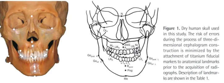
(2) Park et al • Accuracy of biplanar imaging system. INTRODUCTION. therefore, it is the preferred method for the construction of 3D cephalograms.8-12,18 Kusnoto et al.12 demonstrated the clinical validity of a 3D CephTM (Department of Orthodontics, University of Chicago, IL, USA) program for the measurement of 3D distances by combining lateral, frontal, and sub mentovertex cephalograms. In routine practice, the practitioner can obtain frontal and lateral cephalograms by using a single X-ray beam and a rotational radio graphic cassette. However, this requires the patient to change the head posture, which results in the acquisition of images of two different head positions. The biplanar imaging system enables the simultaneous acquisition of frontal and lateral cephalograms at a 90o angle.15-17,19 The lateral and frontal images are obta ined at a precise angle of 90o, with the patient’s head maintained in the same position. Thus, 3D images are reproduced from two X-ray beams emitted from diffe rent angles, resulting in increased accuracy. In the present study, we generated 3D cephalograms from lateral and frontal images obtained using the biplanar imaging system with the 3D CephTM program. Our objective was to evaluate the accuracy of 3D cephalograms constructed using the biplanar imaging system by comparing the obtained measurements with those obtained from 3D cephalograms constructed using conventional radiography and CBCT.. Cephalometry has become a fundamental part of orthodontic practice since its introduction in the field of dentistry, with applications ranging from diagnosis and treatment planning to the evaluation of treatment outcomes. However, conventional cephalograms only provide a two-dimensional (2D) view of three-dimen sional (3D) objects, which is a major limitation of this imaging modality. Possible differences in magnifying scales, geometric distortions, superimposition of struc tures, and potential errors associated with the projecting radiation beam are other problems associated with cephalometry.1-3 Therefore, clinical efforts to achieve 3D information for orthodontic purposes have been made. More recently, the introduction of cone-beam computed tomography (CBCT) in the field of dentistry has provided clinicians with a tool for obtaining a 3D view of objects. Despite the various advantages of CBCT, the increased exposure to ionizing radiation and relatively high costs are disadvantages for both patients (particularly young patients) and clinicians.4-7 For these reasons, several attempts to generate 3D coordinates by reconstructing 2D radiographs such as lateral and frontal cephalograms have been made.8-13 Currently, two methods for the generation of 3D ce phalograms are available, namely the biplanar method, which is based on biplanar geometry (film cassettes are oriented at 90o to each other at the time of expo sure),14,15 and the coplanar method, which is based on convergent geometry.16,17 When the coplanar method is used, the subject is placed in the same physical location and exposed at different time points, with the film cassettes shifted using an automatic cassette changer. However, a dedicated craniofacial stereometric system is required for the coplanar method. The biplanar method, on the other hand, uses lateral and frontal cephalograms that are routinely obtained for orthodontic diagnosis;. MATERIALS AND METHODS Fifteen dry human skulls with a good dentition and intact skeletal structures were obtained from the Department of Oral Anatomy at the School of Den tistry of Chonnam National University. The study was exempted from approval by the Chonnam National University Dental Hospital Institutional Review Board. To minimize the risk of error during the process of 3D cephalogram construction, two different fiducial markers. N CdR. CdL OrR. OrL. MR. U6R. PNS ANS ML Apoint U6L. U1R U1L. Gopost. R. Goinf. L6R R. L6L L1R L1L Bpoint Pog Me. www.e-kjo.org. https://doi.org/10.4041/kjod.2018.48.5.292. Gopost Goinf. L. L. Figure 1. Dry human skull used in this study. The risk of errors during the process of three-di mensional cephalogram cons truction is minimized by the attachment of titanium fiducial markers to anatomical landmarks prior to the acquisition of radi ographs. Description of landmar ks are shown in the Table 1. 293.

(3) Park et al • Accuracy of biplanar imaging system. (“ο” represented the right side and “–” represented the left side) were attached to anatomical landmarks marked on the dry skulls prior to the acquisition of radiographs (Figure 1). The diameter of the “ο” marker was 1 mm, while the length of the “–” marker was 1 mm. Using conventional radiography and biplanar radio graphy, lateral and frontal cephalograms were obtained. Figure 2. The biplanar imaging system used in this study. Two instrumentariums were positioned at a 90° angle and two arrays of X-ray beams were simultaneously projected toward the subject with the head posture remaining iden tical for both lateral and frontal cephalogram acquisition.. A. C. 294. for each skull. For image acquisition, the Frankfort horizontal plane was set parallel to the floor. The distance between the radiation source and the skull was set at 150 cm, while that from the skull to the film was 15 cm. Electric currents were set at 7 to 8 mA, with a voltage of 75 to 85 kVp and an exposure time of 1.6 seconds. Instrumentarium (OrthoCeph ® OC100; Instrumentarium Imaging Ind. Co. Ltd., Tuusula, Finland) was used to obtain the conventional lateral and frontal cephalograms. For the acquisition of frontal cephalograms, the skulls were repositioned at a 90o angle because the X-ray beams during conventional radiography were projected from a single point. For biplanar radiography, two instrumentariums were used. Two arrays of X-ray beams were simultaneously projected toward the skulls, with the head posture remaining identical for both lateral and frontal cephalogram acquisition (Figure 2). The magnification of conventional and biplanar images was 110%. For the purpose of comparison, CBCT-generated cephalograms were also included. A CBCT scanner (Alphard Vega; Asahi Roentgen Co., Kyoto, Japan) was used to generate 3D frontal and lateral images, which were saved using InVivo software (version 5.3; Anatomage, San Jose, CA, USA) for the construction of 3D cephalograms using the “capture to file” function. The frontal and lateral images were colored to enable clearer visualization and easier identification of fiducial markers.. B. D. Figure 3. The three-dimen sional (3D) Ceph TM program (Department of Orthodontics, University of Chicago, IL, USA) used in this study. A and B, Input of lateral and frontal cephalograms into the 3D CephTM program. C, Landmark correction using vector intercept with manual or averaging algorithm in the 3D AlignerTM program (Department of Orthodontics, University of Illinois at Chicago, Chicago, IL, USA). D, Gene ration of a three-dimensional cephalometric image using the “create 3D frame” function and measurement output using the “3D log” function in the program.. https://doi.org/10.4041/kjod.2018.48.5.292. www.e-kjo.org.

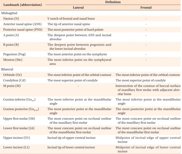
(4) Park et al • Accuracy of biplanar imaging system. Construction of 3D cephalograms Three types of 3D cephalograms were generated from the images obtained using conventional radiography (3D cephconv), the biplanar imaging system (3D cephbiplanar), and CBCT (3D cephcbct). The 3D CephTM program was used to construct 3D cephalograms from the frontal and lateral images generated using the conventional and biplanar imaging methods. When radiographs from different machines were imported into the program, each image size was standardized according to the program settings. Using the program’s calibration tool, two points were identified on the image to represent a distance of 10 mm. Each frontal and lateral cephalogram obtained using each of the three techniques were imported into the 3D Ceph TM program. After 25 landmarks were identified, 3D images were generated by connecting the landmarks marked on the frontal. and lateral images. Using the 3D log function of the 3D Aligner program (Department of Orthodontics, University of Illinois at Chicago, Chicago, IL, USA), the 3D images were transformed and distances between landmarks were calculated (Figure 3). The definitions of the landmarks used in this study are provided in Table 1. For evaluation of the accuracy of 3D cephalograms constructed from 2D images (conventional and biplanar radiographs) by using CBCT-generated cephalograms as a reference, a total of 25 landmarks were decided. Then, 34 measurements, including oblique (n = 15) measurements and measurements for width (n = 7), depth (n = 7), and height (n = 5), were obtained for each skull. For statistical analysis, paired t -tests and Bland– Altman plotting were used. The Shapiro–Wilk test showed normal data distribution. Paired t -tests were conducted at a 5% significance level using SPSS. Table 1. Definitions of cephalometric landmarks used in this study Landmark (abbreviation). Definition Lateral. Frontal. Midsagittal Nasion (N). V notch of frontal and nasal bone. -. Anterior nasal spine (ANS). The tip of anterior nasal spine. -. Posterior nasal spine (PNS). The most posterior point of hard palate. -. A point (A). The deepest point between ANS and incisal alveolus. -. B point (B). The deepest point between pogonion and the lower incisal alveolus. -. Pogonion (Pog). The most anterior point on the symphysis. -. Menton (Me). The most inferior point on the symphyseal area. -. Bilateral Orbitale (Or). The most inferior point of the orbital contour. The most inferior point of the orbital contour. Condylion (Cd). The most superior point of condyle. The most superior point of condyle. M point (M). -. Intersection of the contour of buccal surface of maxillary first molar with adjacent alve olar bone. Gonion inferior (Goinf ). The most inferior point at the mandibular angle. The most inferior point at the mandibular angle. Gonion posterior (Gopost). The most posterior point at the mandibular angle. The most posterior point at the mandibular angle. Upper first molar (U6). The most concave point on occlusal outline of the maxillary first molar. The most concave point on occlusal outline of the maxillary first molar. Lower first molar (L6). The most concave point on occlusal outline of the mandibular first molar. The most concave point on occlusal outline of the mandibular first molar. Upper incisor (U1). Incisal tip of upper central incisor. Midpoint of incisal edge of upper central incisor. Lower incisor (L1). Incisal tip of lower central incisor. Midpoint of incisal edge of lower central incisor. www.e-kjo.org. https://doi.org/10.4041/kjod.2018.48.5.292. 295.

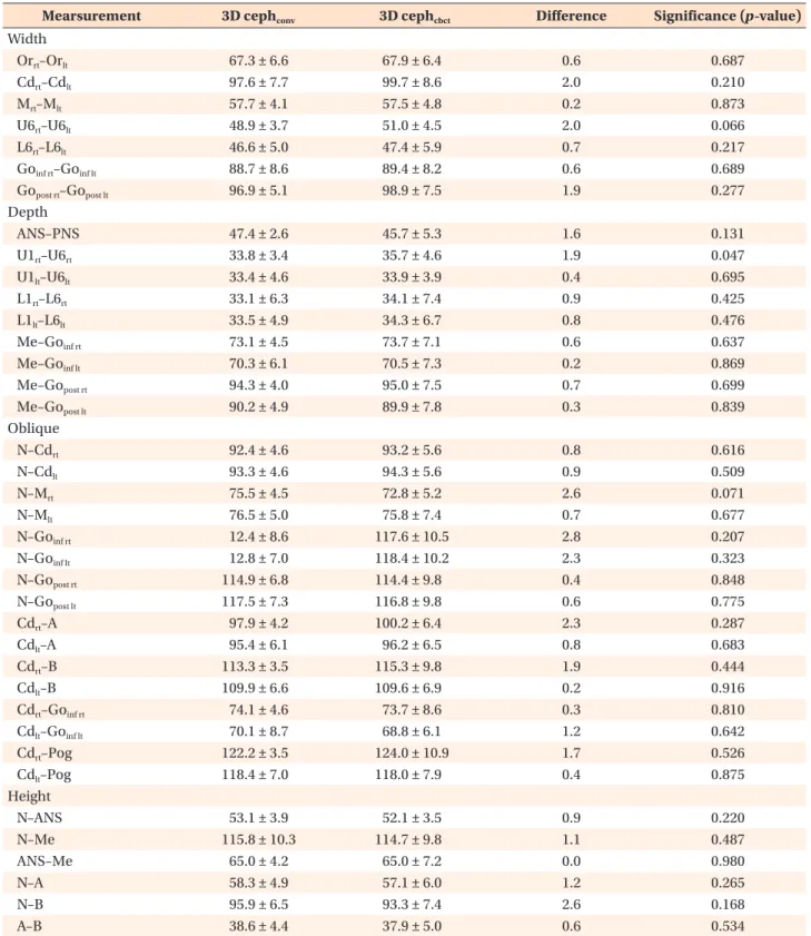
(5) Park et al • Accuracy of biplanar imaging system. Table 2. Comparison between CBCT-generated cephalograms and 3D cephalograms constructed from conventional cephalograms Mearsurement Width Orrt–Orlt Cdrt–Cdlt Mrt–Mlt U6rt–U6lt L6rt–L6lt Goinf rt–Goinf lt Gopost rt–Gopost lt Depth ANS–PNS U1rt–U6rt U1lt–U6lt L1rt–L6rt L1lt–L6lt Me–Goinf rt Me–Goinf lt Me–Gopost rt Me–Gopost lt Oblique N–Cdrt N–Cdlt N–Mrt N–Mlt N–Goinf rt N–Goinf lt N–Gopost rt N–Gopost lt Cdrt–A Cdlt–A Cdrt–B Cdlt–B Cdrt–Goinf rt Cdlt–Goinf lt Cdrt–Pog Cdlt–Pog Height N–ANS N–Me ANS–Me N–A N–B A–B. 3D cephconv. 3D cephcbct. Difference. Significance (p -value). 67.3 ± 6.6 97.6 ± 7.7 57.7 ± 4.1 48.9 ± 3.7 46.6 ± 5.0 88.7 ± 8.6 96.9 ± 5.1. 67.9 ± 6.4 99.7 ± 8.6 57.5 ± 4.8 51.0 ± 4.5 47.4 ± 5.9 89.4 ± 8.2 98.9 ± 7.5. 0.6 2.0 0.2 2.0 0.7 0.6 1.9. 0.687 0.210 0.873 0.066 0.217 0.689 0.277. 47.4 ± 2.6 33.8 ± 3.4 33.4 ± 4.6 33.1 ± 6.3 33.5 ± 4.9 73.1 ± 4.5 70.3 ± 6.1 94.3 ± 4.0 90.2 ± 4.9. 45.7 ± 5.3 35.7 ± 4.6 33.9 ± 3.9 34.1 ± 7.4 34.3 ± 6.7 73.7 ± 7.1 70.5 ± 7.3 95.0 ± 7.5 89.9 ± 7.8. 1.6 1.9 0.4 0.9 0.8 0.6 0.2 0.7 0.3. 0.131 0.047 0.695 0.425 0.476 0.637 0.869 0.699 0.839. 92.4 ± 4.6 93.3 ± 4.6 75.5 ± 4.5 76.5 ± 5.0 12.4 ± 8.6 12.8 ± 7.0 114.9 ± 6.8 117.5 ± 7.3 97.9 ± 4.2 95.4 ± 6.1 113.3 ± 3.5 109.9 ± 6.6 74.1 ± 4.6 70.1 ± 8.7 122.2 ± 3.5 118.4 ± 7.0. 93.2 ± 5.6 94.3 ± 5.6 72.8 ± 5.2 75.8 ± 7.4 117.6 ± 10.5 118.4 ± 10.2 114.4 ± 9.8 116.8 ± 9.8 100.2 ± 6.4 96.2 ± 6.5 115.3 ± 9.8 109.6 ± 6.9 73.7 ± 8.6 68.8 ± 6.1 124.0 ± 10.9 118.0 ± 7.9. 0.8 0.9 2.6 0.7 2.8 2.3 0.4 0.6 2.3 0.8 1.9 0.2 0.3 1.2 1.7 0.4. 0.616 0.509 0.071 0.677 0.207 0.323 0.848 0.775 0.287 0.683 0.444 0.916 0.810 0.642 0.526 0.875. 53.1 ± 3.9 115.8 ± 10.3 65.0 ± 4.2 58.3 ± 4.9 95.9 ± 6.5 38.6 ± 4.4. 52.1 ± 3.5 114.7 ± 9.8 65.0 ± 7.2 57.1 ± 6.0 93.3 ± 7.4 37.9 ± 5.0. 0.9 1.1 0.0 1.2 2.6 0.6. 0.220 0.487 0.980 0.265 0.168 0.534. Values are presented as mean ± standard deviation. CBCT, Cone-beam computed tomography; 3D, three dimensional; cephconv, 3D cephalogram by conventional radiography; cephcbct, 3D cephalogram by CBCT; rt, right; lt, left; post, posterior; inf, inferior. Significance was determined by the paired t -test. Descriptions of landmarks are shown in Figure 1 and Table 1.. 296. https://doi.org/10.4041/kjod.2018.48.5.292. www.e-kjo.org.

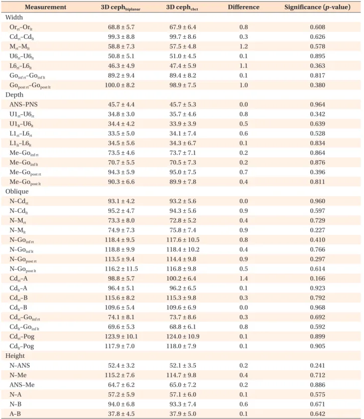
(6) Park et al • Accuracy of biplanar imaging system. Table 3. Comparison between CBCT-generated cephalograms and 3D cephalograms constructed from biplanar cephalograms Measurement Width Orrt–Orlt Cdrt–Cdlt Mrt–Mlt U6rt–U6lt L6rt–L6lt Goinf rt–Goinf lt Gopost rt–Gopost lt Depth ANS–PNS U1rt–U6rt U1lt–U6lt L1rt–L6rt L1lt–L6lt Me–Goinf rt Me–Goinf lt Me–Gopost rt Me–Gopost lt Oblique N–Cdrt N–Cdlt N–Mrt N–Mlt N–Goinf rt N–Goinf lt N–Gopost rt N–Gopost lt Cdrt–A Cdlt–A Cdrt–B Cdlt–B Cdrt–Goinf rt Cdlt–Goinf lt Cdrt–Pog Cdlt–Pog Height N–ANS N–Me ANS–Me N–A N–B A–B. 3D cephbiplanar. 3D cephcbct. Difference. Significance (p -value). 68.8 ± 5.7 99.3 ± 8.8 58.8 ± 7.3 50.8 ± 5.1 46.3 ± 4.9 89.2 ± 9.4 100.0 ± 8.2. 67.9 ± 6.4 99.7 ± 8.6 57.5 ± 4.8 51.0 ± 4.5 47.4 ± 5.9 89.4 ± 8.2 98.9 ± 7.5. 0.8 0.3 1.2 0.1 1.1 0.1 1.0. 0.608 0.626 0.578 0.895 0.363 0.817 0.380. 45.7 ± 4.4 34.8 ± 3.0 34.4 ± 4.2 33.5 ± 5.0 34.5 ± 5.6 73.5 ± 4.6 70.7 ± 5.5 94.3 ± 5.9 90.3 ± 6.6. 45.7 ± 5.3 35.7 ± 4.6 33.9 ± 3.9 34.1 ± 7.4 34.3 ± 6.7 73.7 ± 7.1 70.5 ± 7.3 95.0 ± 7.5 89.9 ± 7.8. 0.0 0.8 0.5 0.6 0.1 0.2 0.2 0.7 0.4. 0.964 0.342 0.639 0.528 0.834 0.864 0.876 0.396 0.811. 93.1 ± 4.2 95.2 ± 4.7 73.3 ± 8.0 74.9 ± 7.3 118.4 ± 9.5 118.8 ± 9.9 113.5 ± 9.4 116.2 ± 11.5 98.8 ± 5.7 96.4 ± 5.1 115.6 ± 8.2 109.6 ± 5.4 74.1 ± 8.1 69.6 ± 5.3 123.9 ± 10.1 117.9 ± 7.0. 93.2 ± 5.6 94.3 ± 5.6 72.8 ± 5.2 75.8 ± 7.4 117.6 ± 10.5 118.4 ± 10.2 114.4 ± 9.8 116.8 ± 9.8 100.2 ± 6.4 96.2 ± 6.5 115.3 ± 9.8 109.6 ± 6.9 73.7 ± 8.6 68.8 ± 6.1 124.0 ± 10.9 118.0 ± 7.9. 0.0 0.9 0.4 0.9 0.8 0.4 0.9 0.5 1.4 0.1 0.3 0.0 0.3 0.8 0.1 0.1. 0.960 0.597 0.729 0.227 0.410 0.766 0.297 0.614 0.166 0.923 0.792 0.968 0.692 0.592 0.899 0.905. 52.4 ± 3.2 115.2 ± 7.6 64.7 ± 6.2 57.2 ± 5.9 94.0 ± 6.8 37.8 ± 4.5. 52.1 ± 3.5 114.7 ± 9.8 65.0 ± 7.2 57.1 ± 6.0 93.3 ± 7.4 37.9 ± 5.0. 0.2 0.4 0.2 0.1 0.6 0.1. 0.241 0.712 0.886 0.575 0.671 0.642. Values are presented as mean ± standard deviation. CBCT, Cone-beam computed tomography; 3D, three dimensional; cephbiplanar, 3D cephalogram by biplanar imaging system; cephcbct, 3D cephalogram by CBCT; rt, right; lt, left; post, posterior; inf, inferior. Significance was determined by the paired t -test. Descriptions of landmarks are shown in Figure 1 and Table 1.. www.e-kjo.org. https://doi.org/10.4041/kjod.2018.48.5.292. 297.

(7) Park et al • Accuracy of biplanar imaging system. software (version 20; IBM Co., Armonk, NY, USA), while Bland–Altman plotting was performed using MedCalc statistical software (Ostend, Belgium).. RESULTS The mean and standard deviation values for each measurement recorded on 3D cephalograms generated from conventional radiographs and CBCT images are shown in Table 2. Differences in measurements for width, height, and depth ranged from 0.1 to 2.6 mm, while differences in oblique measurements ranged from 0.2 to 2.8 mm. Overall, differences in oblique measurements were greater than those in measurements for width, height, and depth. Paired t -tests were used to compare measurements between the two image sets; the results revealed no significant differences (Table 2). Table 3 lists the measurements recorded on biplanar 3D cephalograms and CBCT-generated cephalograms. Differences in measurements for height and width ranged from 0.1 to 0.6 mm and from 0.1 to 1.2 mm, respectively. With regard to oblique measurements, differences ranged from 0.0 to 1.4 mm. The results of paired t -tests revealed no significant differences between the two image sets (Table 3). The findings of Bland–Altman plotting showed no systematic differences in measurements between the biplanar 3D cephalograms and CBCT-generated cephalograms (Tables 4 and 5). The magnitude of differences was not large and mostly within a 95% confidence interval (Figure 4).. DISCUSSION In the present study, we evaluated the accuracy of 3D cephalograms generated using a biplanar imaging system by comparing obtained measurements with those recorded on 3D cephalograms constructed from conventional radiographs and CBCT images. The results revealed no significant differences in measurements among the three image sets, although the cephalograms constructed from conventional radiographs showed larger deviations than those constructed using the biplanar imaging system when CBCT measurements were used as a reference. Kusnoto et al.12 found that different head orientations and tracing errors could affect the accuracy of 3D cephalograms. In the present study, we used 25 fiducial markers as right, left, and midline anatomical landmarks on the skull in order to minimize landmark identification errors. The use of radiopaque titanium markers enables the accurate digitization of landmarks in both lateral and frontal projections. During the process of 3D cephalogram construction, obtained coordinates of projected object points are. 298. Table 4. Bland–Altman analysis of the accuracy of threedimensional measurements obtained from conventional cephalograms Measurement Width Orrt–Orlt Cdrt–Cdlt Mrt–Mlt U6rt–U6lt L6rt–L6lt Goinf rt–Goinf lt Gopost rt–Gopost lt Depth ANS–PNS U1rt–U6rt U1lt–U6lt L1rt–L6rt L1lt–L6lt Me–Goinf rt Me–Goinf lt Me–Gopost rt Me–Gopost lt Oblique N–Cdrt N–Cdlt N–Mrt N–Mlt N–Goinf rt N–Goinf lt N–Gopost rt N–Gopost lt Cdrt–A Cdlt–A Cdrt–B Cdlt–B Cdrt–Goinf rt Cdlt–Goinf lt Cdrt–Pog Cdlt–Pog Height N–ANS N–Me ANS–Me N–A N–B A–B. Bias. Limit of agreement. Agreement width. −0.63 −2.08 0.22 −2.09 −0.79 −0.65 −1.99. −12.23 to 10.98 −14.09 to 9.93 −10.04 to 10.49 −10.05 to 5.87 −5.45 to 3.86 −12.76 to 11.46 −15.36 to 11.38. 23.21 24.02 20.53 15.92 9.31 24.22 26.74. 1.62 −0.73 −0.41 −0.98 −0.84 −0.65 −0.22 −0.73 0.34. −6.68 to 9.91 −14.80 to 13.34 −8.20 to 7.38 −10.03 to 8.07 −9.59 to 7.90 −10.94 to 9.63 −10.19 to 9.75 −14.80 to 13.34 −12.00 to 12.68. 16.59 28.14 15.58 18.10 17.49 20.57 19.94 28.14 24.68. −0.82 −0.94 2.69 0.71 2.82 2.40 0.44 0.68 −2.33 −0.85 −1.98 0.28 0.40 1.26 −1.78 0.45. −13.02 to 11.37 −11.48 to 9.60 −7.78 to 13.16 −11.97 to 13.40 −13.33 to 18.97 −15.37 to 20.17 −16.75 to 17.64 −16.97 to 18.32 −18.29 to 13.64 −16.32 to 14.62 −21.08 to 17.11 −19.08 to 19.63 −11.95 to 12.75 −18.95 to 21.48 −22.64 to 19.07 −20.71 to 21.60. 24.39 21.08 20.94 25.37 32.30 35.54 34.39 35.29 31.93 30.94 38.19 38.71 24.70 40.43 41.71 42.31. 0.95 −1.12 −0.04 −1.24 2.62 0.66. −4.65 to 6.54 −12.97 to 10.74 −10.31 to 10.24 −9.32 to 6.85 −11.05 to 16.29 −7.24 to 8.57. 11.19 23.71 20.55 16.17 27.34 15.81. A positive value of bias indicates that three-dimensional measurements obtained from conventional cephalograms are larger than those obtained from cone-beam computed tomography images. rt, Right; lt, left; post, posterior; inf, inferior. Descriptions of landmarks are shown in Figure 1 and Table 1.. https://doi.org/10.4041/kjod.2018.48.5.292. www.e-kjo.org.

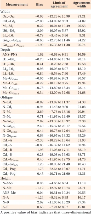
(8) Park et al • Accuracy of biplanar imaging system. Table 5. Bland–Altman analysis of the accuracy of threedimensional measurements obtained from biplanar ce phalograms Measurement Width Orrt–Orlt Cdrt–Cdlt Mrt–Mlt U6rt–U6lt L6rt–L6lt Goinf rt–Goinf lt Gopost rt–Gopost lt Depth ANS–PNS U1rt–U6rt U1lt–U6lt L1rt–L6rt L1lt–L6lt Me–Goinf rt Me–Goinf lt Me–Gopost rt Me–Gopost lt Oblique N–Cdrt N–Cdlt N–Mrt N–Mlt N–Goinf rt N–Goinf lt N–Gopost rt N–Gopost lt Cdrt–A Cdlt–A Cdrt–B Cdlt–B Cdrt–Goinf rt Cdlt–Goinf lt Cdrt–Pog Cdlt–Pog Height N–ANS N–Me ANS–Me N–A N–B A–B. Bias. Limit of agreement. Agreement width. 0.88 −0.33 1.27 −0.18 −1.12 −0.15 1.08. −11.82 to 13.58 −5.40 to 4.74 −15.69 to 18.23 −10.42 to 10.06 −10.17 to 7.92 −4.91 to 4.62 −7.98 to 10.14. 25.40 10.15 33.92 20.48 18.09 9.53 18.12. −0.03 −0.88 0.51 −0.66 0.20 −0.25 0.25 −0.73 0.40. −4.64 to 4.59 −7.72 to 5.95 −7.49 to 8.50 −8.41 to 7.09 −6.89 to 7.29 −11.25 to 10.75 −11.74 to 12.24 −7.04 to 5.59 −12.16 to 12.97. 9.23 13.67 15.99 15.50 14.18 22.00 23.98 12.63 25.13. −0.09 0.96 0.45 −0.94 0.80 0.46 −0.95 −0.57 −1.46 0.14 0.32 0.05 0.36 0.81 −0.14 −0.15. −13.27 to 13.09 −12.46 to 14.38 −9.30 to 10.21 −6.56 to 4.69 −6.38 to 7.98 −10.91 to 11.82 −7.62 to 5.72 −8.99 to 7.85 −9.06 to 6.14 −10.58 to 10.86 −8.59 to 9.22 −9.60 to 9.70 −6.47 to 7.20 −10.43 to 12.05 −7.77 to 7.49 −9.42 to 9.13. 26.36 26.84 19.51 11.25 14.36 22.73 13.34 16.84 15.20 21.44 17.81 19.30 13.67 22.48 15.26 18.55. 0.27 0.49 0.23 0.15 0.69 −0.17. −1.42 to 1.97 −9.45 to 10.44 −14.51 to 14.97 −1.86 to 2.16 −11.43 to 12.82 −2.92 to 2.57. 3.39 19.89 29.48 4.02 24.25 5.49. A positive value of bias indicates that three-dimensional measurements obtained from biplanar cephalograms are larger than those obtained from cone-beam computed tomography images. rt, Right; lt, left; post, posterior; inf, inferior. Descriptions of landmarks are shown in Figure 1 and Table 1.. www.e-kjo.org. https://doi.org/10.4041/kjod.2018.48.5.292. matched using one of two algorithms: vector intercept with averaging algorithm 8,12 or vector intercept with manual adjustment algorithm .9 Both algorithms use the vector principle for the location of landmarks in space. These two algorithms have been shown to have the same degree of accuracy for linear measurements under minimal head rotation and landmark identification errors.8 The only difference between the two algorithms is the involvement of the operator for landmark iden tification. In the vector intercept with manual adju stment algorithm, the operator can manually correct misidentified landmarks during the process. Although such manual adjustment allows the operator to adjust misidentified landmarks, it is time consuming and inconvenient for quick analysis. The vector intercept with averaging algorithm automatically takes the midpoint of landmarks on two planes (frontal and lateral). Therefore, it is easier to use and less time consuming. In the present study, landmarks were identified with the vector intercept with averaging algorithm.8,20 For the acquisition of lateral and frontal cephalograms, a single X-ray beam and rotational radiographic cas settes are normally used. However, the patient’s head position needs to be changed for this conventional approach, which results in images of different head positions. The biplanar imaging system allows the simultaneous acquisition of frontal and lateral images at a precise angle of 90 o angle, without requiring a change in the patient’s head position. Thus, 3D images reproduced from two X-ray beams emitted from different angles could have the same geometry. By comparing 3D measurements obtained using conventional and biplanar radiography with those obtained using CBCT, we aimed to prove the accuracy and clinical validity of the biplanar imaging system. Biplanar radiography used an anteroposterior (AP) projection instead of a posteroanterior (PA) projection, because the former is required for composite imaging with clinical facial photographs for further study. According to Na’s study,21 differences in identification errors between the AP and PA projections were not statistically significant for any landmark. The magnification of images obtained from conventional and biplanar radiography is 110%. In the present study, we compared 3D cephalograms generated using conventional and biplanar radiography with CBCT-generated cephalograms. While the conventional and biplanar cephalograms were perspective view images with a 150/15-cm setting, the CBCT-generated cephalograms were orthogonal view images which could be used as a reference with direct measurements on the skull. In the present study, all measurements obtained from biplanar cephalograms showed no statistically significant differences when compared with measurements obta. 299.

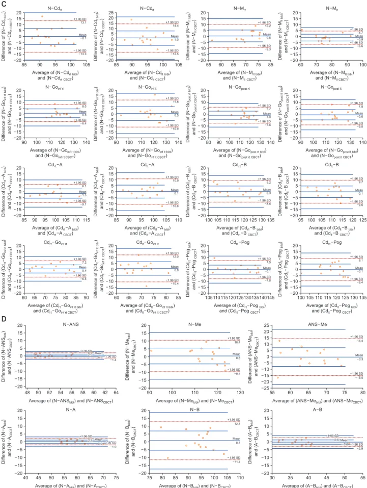
(9) Park et al • Accuracy of biplanar imaging system. Figure 4. Bland–Altman plots for the comparison of three-dimensional (3D) cephalograms constructed from biplanar radiographs and cone-beam computed tomography (CBCT) images. The x-axis shows the average measurements obtained from biplanar cephalograms and CBCT-generated cephalograms, whereas the y-axis represents differences in measurements between the two image sets. The red line represents standard deviations and the blue line represents the upper and lower limits of agreement. A, Width measurements; B, depth measurements; C, oblique measurements; D, height measurements. Descriptions of landmarks are shown in Figure 1 and Table 1. ined from conventional radiograph- and CBCTgenerated cephalograms. These results indicated that biplanar radiography enables the acquisition of lateral and frontal projections with the same geometry, which results in accurate orthogonal projections. Therefore, clinicians can utilize these 3D cephalograms for various analyses, without the requirement for CBCT. Paired t -tests and Bland–Altman analysis revealed that plots were distributed over a wide area, which meant that there were no consistent patterns. Thus, the results were not significantly different.22,23 Most data, with the exception of one or two measurements, were within 95% confidence intervals and distributed within the limits of agreement. While the 3D cephalograms constructed from conven tional radiographs showed larger deviations than did the 3D cephalograms constructed from biplanar images, both image sets were comparable with CBCT-generated cephalograms with regard to all parameters except one. These findings suggest that conventional radiography can be used as an alternative to biplanar radiography.. 300. However, in the present study, the subjects were skulls and not living patients. Moreover, the skulls were fixed in a cephalostat, with the Frankfort plane parallel to the floor. Therefore, errors in the head position or head movement were minimized. In the clinical setting, diffe rent head orientations and tracing errors could affect the accuracy of 3D cephalograms constructed from conventional radiographs.12. CONCLUSION Although measurements recorded on 3D cephalograms constructed from conventional radiographs showed no significant differences from those recorded on CBCTgenerated cephalograms, they showed larger devia tions than measurements recorded on biplanar 3D cephalograms. Thus, more accurate 3D cephalograms can be constructed from biplanar radiographs than from conventional radiographs. Moreover, the biplanar imaging technique may be a useful alternative to CBCT for clinical procedures such as 3D analysis of. https://doi.org/10.4041/kjod.2018.48.5.292. www.e-kjo.org.

(10) Park et al • Accuracy of biplanar imaging system. Figure 4. Continued. facial asymmetry. In conclusion, the findings of this study suggest that 3D reconstruction of 2D biplanar radiographs is a useful clinical technique to obtain 3D information without the use of CBCT.. CONFLICTS OF INTEREST No potential conflict of interest relevant to this article was reported.. ACKNOWLEDGEMENTS This research was supported by Basic Science Research Program through the National Research Foundation of Korea (NRF) funded by the Ministry of Science, ICT & Future Planning (NRF-2014R1A1A1003559). This research was supported by Basic Science Research Program through the National Research Foundation of Korea (NRF) funded by the Ministry of Education (NRF2017R1D1A1B03032132).. www.e-kjo.org. https://doi.org/10.4041/kjod.2018.48.5.292. REFERENCES 1. Bergersen EO. Enlargement and distortion in cepha lometric radiography: compensation tables for linear measurements. Angle Orthod 1980;50:230-44. 2. Ahlqvist J, Eliasson S, Welander U. The cephalome tric projection. Part II. Principles of image distortion in cephalography. Dentomaxillofac Radiol 1983;12: 101-8. 3. Jung PK, Lee GC, Moon CH. Comparison of conebeam computed tomography cephalometric measurements using a midsagittal projection and conventional two-dimensional cephalometric measurements. Korean J Orthod 2015;45:282-8. 4. Farman AG. ALARA still applies. Oral Surg Oral Med Oral Pathol Oral Radiol Endod 2005;100:395-7. 5. American Dental Association Council on Scientific Affairs. The use of cone-beam computed tomogra phy in dentistry: an advisory statement from the American Dental Association Council on Scientific. 301.

(11) Park et al • Accuracy of biplanar imaging system. Figure 4. Continued. 302. https://doi.org/10.4041/kjod.2018.48.5.292. www.e-kjo.org.

(12) Park et al • Accuracy of biplanar imaging system. Affairs. J Am Dent Assoc 2012;143:899-902. 6. American Academy of Oral and Maxillofacial Radiology. Clinical recommendations regarding use of cone beam computed tomography in ortho dontics. [corrected]. Position statement by the American Academy of Oral and Maxillofacial Radio logy. Oral Surg Oral Med Oral Pathol Oral Radiol 2013;116:238-57. 7. Abdelkarim AA. Appropriate use of ionizing radiation in orthodontic practice and research. Am J Orthod Dentofacial Orthop 2015;147:166-8. 8. Grayson B, Cutting C, Bookstein FL, Kim H, McCar thy JG. The three-dimensional cephalogram: Theory, techniques, and clinical application. Am J Orthod Dentofacial Orthop 1988;94:327-37. 9. Brown T, Abbott AH. Computer-assisted location of reference points in three dimensions for radiographic cephalometry. Am J Orthod Dentofacial Orthop 1989;95:490-8. 10. Trocmé MC, Sather AH, An KN. A biplanar cephalo metric stereoradiography technique. Am J Orthod Dentofacial Orthop 1990;98:168-75. 11. Bookstein FL, Grayson B, Cutting CB, Kim HC, McCarthy JG. Landmarks in three dimensions: reconstruction from cephalograms versus direct observation. Am J Orthod Dentofacial Orthop 1991; 100:133-40. 12. Kusnoto B, Evans CA, BeGole EA, de Rijk W. Asse ssment of 3-dimensional computer-generated ce phalometric measurements. Am J Orthod Dento facial Orthop 1999;116:390-9. 13. Mori Y, Miyajima T, Minami K, Sakuda M. An accurate three-dimensional cephalometric sys tem: a solution for the correction of cephalic mal positioning. J Orthod 2001;28:143-9. 14. Suh CH. The fundamentals of computer aided X-ray. www.e-kjo.org. https://doi.org/10.4041/kjod.2018.48.5.292. analysis of the spine. J Biomech 1974;7:161-9. 15. Selvik G, Alberius P, Fahiman M. Roentgen stereo photogrammetry for analysis of cranial growth. Am J Orthod 1986;89:315-25. 16. Baumrind S, Moffitt FH, Curry S. Three-dimensional x-ray stereometry from paired coplanar images: A progress report. Am J Orthod Dentofacial Orthop 1983;84:292-312. 17. Baumrind S, Moffitt FH, Curry S. The geometry of three-dimensional measurement from paired coplanar x-ray images. Am J Orthod 1983;84:31322. 18. Cutting C, Bookstein FL, Grayson B, Fellingham L, McCarthy JG. Three-dimensional computer-assi sted design of craniofacial surgical procedures: optimization and interaction with cephalometric and CT-based models. Plast Reconstr Surg 1986;77:87787. 19. Selvik G. Roentgen stereophotogrammetric analysis. Acta Radiol 1990;31:113-26. 20. Bae GS, Park SB, Son WS. The comparative study of three-dimensional cephalograms to actual models and conventional lateral cephalograma in linear and angular measurements. Korean J Orthod 1997;27:129-40. 21. Na ER. Comparison of landmark identification errors between postero-anterior and antero-posterior cephalograms generated from cone-beam CT scan data [PhD dissertation]. Gwangju, Korea: Chonnam National University of Korea; 2013. 22. Bland JM, Altman DG. Statistical methods for assessing agreement between two methods of clinical measurement. Lancet 1986;327:307-10. 23. Bland JM, Altman DG. Measuring agreement in method comparison studies. Stat Methods Med Res 1999;8:135-60.. 303.

(13)