Landslide Susceptibility Prediction using Evidential Belief Function, Weight of Evidence and Artificial Neural Network Models

Korean Journal of Remote Sensing, Vol.35, No.2, 2019, pp.299~316

https://doi.org/10.7780/kjrs.2019.35.2.9 ISSN 1225-6161 ( Print )

ISSN 2287-9307 (Online)

Article

Evidential Belief Function, Weight of Evidence 및 Artificial Neural Network 모델을 이용한

산사태 공간 취약성 예측 연구

이사로 ^1),2)·오현주 ^3)†

Landslide Susceptibility Prediction using Evidential Belief Function, Weight of Evidence and Artificial Neural Network Models

Saro Lee

·Hyun-Joo Oh

Abstract: The purpose of this study was to analyze landslide susceptibility in the Pyeongchang area using Weight of Evidence (WOE) and Evidential Belief Function (EBF) as probability models and Artificial Neural Networks (ANN) as a machine learning model in a geographic information system (GIS). This study examined the widespread shallow landslides triggered by heavy rainfall during Typhoon Ewiniar in 2006, which caused serious property damage and significant loss of life. For the landslide susceptibility mapping, 3,955 landslide occurrences were detected using aerial photographs, and environmental spatial data such as terrain, geology, soil, forest, and land use were collected and constructed in a spatial database. Seventeen factors that could affect landsliding were extracted from the spatial database. All landslides were randomly separated into two datasets, a training set (50%) and validation set (50%), to establish and validate the EBF, WOE, and ANN models. According to the validation results of the area under the curve (AUC) method, the accuracy was 74.73%, 75.03%, and 70.87% for WOE, EBF, and ANN, respectively. The EBF model had the highest accuracy. However, all models had predictive accuracy exceeding 70%, the level that is effective for landslide susceptibility mapping. These models can be applied to predict landslide susceptibility in an area where landslides have not occurred previously based on the relationships between landslide and environmental factors.

This susceptibility map can help reduce landslide risk, provide guidance for policy and land use

Received April 5, 2019; Revised April 14, 2019; Accepted April 18, 2019; Published online April 25, 2019

1)

한국지질자원연구원 지오플랫폼연구본부 책임연구원 (Principal Researcher, Geoscience Platform Research Division, Korea Institute of Geoscience and Mineral Resources)

2)

과학기술연합대학원대학교 물리탐사공학과 정교수 (Professor, Department of Geophysical Exploration, University of Science and Technology)

3)

한국지질자원연구원 지질환경연구본부 선임연구원 (Senior Researcher, Geologic Environment Division, Korea Institute of Geoscience and Mineral Resources)

†

Corresponding Author: Hyun-Joo Oh ([email protected])

This is an Open-Access article distributed under the terms of the Creative Commons Attribution Non-Commercial License

(http://creativecommons.org/licenses/by-nc/3.0) which permits unrestricted non-commercial use, distribution, and reproduction in

any medium, provided the original work is properly cited.

1. 서 론

GIS 및 다양한 모델의 사용이 증가하면서 산사태 취 약성을 평가하기 위한 많은 모델이 제안되었고, 특히 최 근에는 많은 연구에서 GIS를 이용한 확률, 통계, 머신러 닝 및 이들의 융합 모델과 같은 다양한 모델이 적용되 었다 (Lee, 2019). 확률 모델에서는 빈도비 모델(Lee and Pradhan, 2006; Li et al., 2017; Oh et al., 2017; Razavizadeh et

2013; Tsangaratos et al., 2017), EBF 모델(Althuwaynee et

2013), statistical index 모델(Chen et al., 2018b; Hong et al., 2018; Pham et al., 2017; Pham et al., 2019), logistic regression 모델(Althuwaynee et al., 2014b; Choi et al., 2012; Kalantar et

등이 많이 적용되었다 . 또한 기계학습 모델 중에서는 fuzzy logic 모델(Bui et al., 2015; Fatemi Aghda et al., 2018;

Feizizadeh et al., 2017; Lee, 2007; Pourghasemi et al., 2012), fuzzy rule-based classifier 모델(Mezaal and Pradhan, 2018;

Pham et al., 2016), neuro fuzzy 모델(Chen et al., 2017a;

Jaafari et al., 2019; Lee et al., 2015a; Oh and Pradhan, 2011;

Pradhan, 2013; Song et al., 2012), multivariate adaptive regression splines(MARS) 모델(Chu et al., 2019; Conoscenti

2018) neural networks 모델(Chen et al., 2017c; Choi et al., 2012; Dou et al., 2015; Kalantar et al., 2018; Pradhan and Lee, 2010; Song et al., 2012), support vector machines 모델(Chen

2018) 등이 적용되었다.

산사태로 인한 재산 및 인명 피해는 국내뿐 아니라 전 세계적으로 계속 발생하고 있으며 , 특히 기상변화로 인한 집중호우로 재산 및 인명 피해가 증가하고 있다 . 따라서 본 연구의 목적은 기초연구로 산사태로 인한 피 해를 최소화하기 위해 산사태 발생 취약 지역을 지도화 하여 예측하는 것이다 . 연구지역은 2006년 태풍 에위니 아로 인한 집중호우로 산사태가 많이 발생한 평창 지역 으로 설정하고 , GIS 기반의 확률 모델인 Weight of Evidence(WOE), Evidential Belief Function(EBF) 및 기계 학습 모델인 Artificial Neural Networks(ANN) 모델을 적 용 및 검증 비교하였다 .

development, and save time and expense for landslide hazard prevention. In the future, more generalized models should be developed by applying landslide susceptibility mapping in various areas.

Key Words: Landslide, Evidential Belief Function, Weight of Evidence, Artificial Neural Network, GIS

요약 : 본 연구는 지리정보시스템 (GIS) 환경에서 확률 모델인 Weight Of Evidence (WOE)와 Evidential Belief

Function (EBF), 기계학습 모델인 Artificial Neural Networks (ANN) 모델을 이용하여 평창지역의 산사태 취약성

도를 공간적으로 분석하고 예측하였다 . 본 연구지역은 2006년 태풍 에위니아에 의한 집중호우로 산사태가 많

이 발생하여 많은 재산 및 인명피해가 발생하였다 . 산사태 취약성도를 작성하기 위해 항공사진을 이용하여

3,955개의 방대한 산사태 발생 위치를 탐지하였고, 환경공간정보인 지형, 지질, 토양, 산림 및 토지이용 등의 공

간 데이터를 수집하여 공간데이터베이스에 구축하였다 . 이러한 공간데이터베이스를 이용하여 산사태에 영향

을 줄 수 있는 인자 17개를 추출하여 입력 인자와 EBF, WOE, ANN 모델을 이용하여 산사태 취약성도를 작성

하고 검증하였다 . 작성 및 검증을 위해 산사태 자료는 각각 50%씩 나누어서 훈련 및 검증을 실시하였고, 검증

결과 WOE 모델의 경우는 74.73%, EBF 모델의 경우는 75.03%, ANN 모델의 경우는 70.87%의 예측 정확도를

나타내었다 . 본 연구에 사용된 모델 중 EBF 모델이 가장 높은 정확도를 나타냈으며, 모든 모델에서 70% 이상

의 예측 정확도를 보여 본 연구에서 사용된 기법이 산사태 취약성도 작성에 유효함을 나타내었다 . 본 연구에서

제안된 WOE, EBF, ANN 모델과 산사태 취약성도는 이전에 산사태가 발생하지 않은 지역의 산사태를 예측하

는 데 사용될 수 있다 . 이러한 취약성도는 산사태 위험 감소를 촉진하고, 토지 이용 정책 및 개발을 위한 기초자

료 역할을 할 수 있으며 , 궁극적으로 산사태 재해 예방을 위한 시간과 비용을 절약할 수 있다. 향후 보다 많은

지역에서 산사태 취약성도 작성 방법을 적용하여 산사태 위험 예측을 위한 일반화된 모델을 이끌어 내야 한다 .

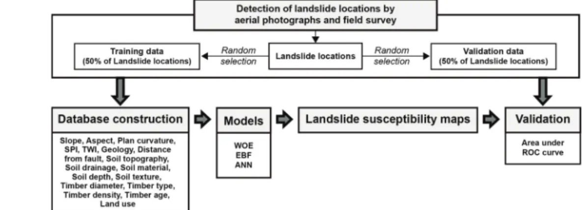
본 연구 흐름은 Fig. 1과 같다: (1) 웹 기반 디지털 항공 사진(http://map.daum.net)에서 3,955개의 방대한 산사태 위치를 탐지하고 현장에서 위치를 확인하였다(Fig. 2).

(2) 산사태 데이터를 훈련용 자료(산사태 위치의 50%) 와 검증용 자료(산사태 위치의 50%)로 무작위로 나누 었다. (3) 환경공간정보인 지형, 토양, 산림, 지질 및 토 지피복 공간 데이터베이스로부터 토양 배수량, 토양 두께, 토양 질감, 산림종류, 산림연령, 산림지름, 산림 밀도 , 단층으로부터의 거리, 경사각, 곡면, 곡률, 지형 습 윤지수 , 지질, 토지이용 등 총 17개의 잠재적으로 산사 태 발생에 기여하는 요인들을 추출하였다 . (4) 훈련을 위해 선택된 WOE, EBF, ANN 모델과 산사태 위치를 이용하여 산사태와 각 요인 간의 관계를 정량적으로 계 산한 후 그 관계를 이용하여 산사태 취약성도를 작성하 였다 . (5) 마지막으로 훈련에 사용되지 않은 검증용 산 사태 위치를 이용하여 산사태 취약성 지도를 검증하여 예측 정확도를 계산하였다 .

2. 연구자료

본 연구지역 (Fig. 2)의 약 65%는 해발 700 m 이상인 고원에 위치하고 있으며 , 평균 기온은 매년 10.3°C, 1월 -6.3°C, 8월에는 24.5°C이며, 연평균 강우량은 1,082 mm 이다 . 본 지역의 지질은 대부분 대보조산운동 때 형성 된 임계화강암으로 이루어져 있다 .

본 연구를 위해 먼저 항공사진을 이용하여 산사태 위 치를 탐지하였다 . 이러한 항공사진의 시각적인 해석은 최근까지 (Kääb, 2002; Casson et al., 2003; Martha et al.,

Fig. 1. Study flow for landslide susceptibility mapping using WOE, EBF and ANN models.

Fig. 2. Detection of landslide occurrence based on

digital aerial photographs with a ground

resolution of 50 cm taken in May 2008

(available online at www.daum.net). (a), (b),

and (c) represent areas where landslides

occurred frequently in the study area.

2010) 산사태 위치 지도화에 대한 주요 접근법이었다. 본 항공사진은 삼아항업에서 UltraCam-X 센서(Microsoft, Graz, Austria)를 사용하여 산사태 발생 시점인 2006년 7월 이후인 2008년에 촬영한 해상도 50cm의 사진을 사 용하였다 (http://www.daum.net). 연구지역 내 집중호우 에 의해 유발된 대부분의 산사태는 규모는 대략 20~40 m, 너비는 2~10 m, 깊이는 1 m 미만이다. 산사태의 위 치표시는 산사태가 발생한 시작점으로 표시하였고 , 연 구지역 내 항공사진을 통해 표시된 전체 산사태 건수는 3,955건으로(Fig. 2) 이는 기존의 연구에 비해 매우 방대 한 양의 산사태 개수이다 . 각 산사태의 위치는 10 m×10 m의 픽셀로 표기하였으며 산사태 데이터는 무작위로 훈련용 자료 (전체 산사태의 50%: 1,978개)와 검증용 자 료 (나머지 50%: 1,977개)로 나누었다.

산사태는 복잡한 요인의 상호 작용으로 발생한다 . 요 인 선택과 해당 자료의 준비는 산사태 취약성도 작성에 매우 중요하다 . 산사태 발생에 영향을 주는 요인은 암 석학 , 지질 구조, 지진, 사면 경사, 지형, 사면에서의 강 우강도 , 지하수 조건, 기후, 식물 피복, 토지 이용 및 인 간 활동을 포함한다 . 이 연구는 이러한 요인 중 이용 가 능한 공간데이터베이스를 통해 환경공간정보인 지형 , 지질 , 토지 이용, 산림 및 토양 요인 등을 추출하였다 (Table 1).

먼저 국토지리정보원 (NGII)에서 발행한 1:5,000 지 형도의 5 m 간격 등고선을 이용하여 10 m x 10 m 해상

도의 디지털 고도 모델 (DEM)이 계산되었다. 선형구조 는 광범위한 경험을 가진 구조 지질학자에 의한 음영기 복도의 해석을 통해 추출되었다 . 지질, 산림 및 토양 정 보는 각각 한국지질자원연구원 (KIGAM), 한국산림과 학원 (KFRI), 국립농업과학원(NAAS)에서 제공되는 1:50,000, 1:25,000, 1:25,000의 축척으로 지질도, 임상도, 토양도에서 추출하였다 . 환경부(ME)에서 발행한 토지 이용도는 2007년 11월에 촬영된 panchromatic Système Probatoire d’Observation de Terre 5(SPOT-5) 영상을 이 용하여 작성되었다 .

DEM을 사용하여 경사도, 경사방향, 곡률, 지형습윤 지수 (TWI) 및 하천파워지수(SPI)를 계산하였다. 지형은 토양 수분 , 지하수 흐름 및 경사 안정성과 같은 수문 조 건의 공간적 변화에 중요한 역할을 한다 . 지형 지표는 공간적 토양 수분 패턴을 묘사하는데 사용된다 (Moore

내에서의 안정성을 높이는 요인으로 고려된다 . SPI는 지형 표면의 주어진 지점에서 잠재적인 흐름 침식을 설 명하는 데 사용할 수 있다 . 유역 면적과 경사가 증가함 에 따라 상향 경사 지역과 수류 속도에 기여하는 물의 양이 증가하고 , 따라서 하천력 지수와 침식 위험이 증 가한다 (Florinsky, 2012).

다양한 암상의 경우 강도 , 구성 및 구조와 같은 다양 한 특성을 가지며 산사태에 대한 저항을 일으키기 때문 에 임상 정보는 산사태 발생에 중요한 역할을 한다 Table 1. Data layer related to landslide of study area

Category Factors Data Type Scale Source

Topographic map

Slope Aspect Plan curvature

TWI SPI

GRID 1:5,000 NGII

Geological map Geology

Distance from fault Polygon 1:50,000 KIGAM

Land use map Land use Polygon 1:5,000 ME

Forest map

Timber diameter Timber type Timber density

Timber age

Polygon 1:25,000 KFRI

Soil map

Soil topography Soil drainage Soil material Soil depth Soil texture

Polygon 1:25,000 NAAS

(Kincal et al., 2009; Chauhan et al., 2010). 단층은 지각 변 동으로 인한 암석의 구조적 취성 변형의 표식으로 , 산 사태가 쉽게 발생한다 . 산사태의 발생은 언덕 경사면의 안정성을 나타내는 지표인 토지 이용 패턴에 따라 다르 다 (Anbalagan, 1992). 산림 피복과 토양 특성은 지표 침 식의 증가 , 산 경사의 변화 및 산사태 발생의 증가를 포 함한 다양한 지형학적 과정에 영향을 미친다 (Edeso et

암상은 지질도 공간데이터베이스에서 추출되었고 , 산 림의 종류 , 지름, 나이, 밀도는 임상도 공간데이터베이 스에서 추출되었으며 , 지형종류, 토성, 토양 배수, 토양 모재 , 토양두께는 토양도 공간데이터베이스에서 추출 되었다 .

이렇게 계산되고 공간데이터베이스에서 추출된 요 인은 총 17개이다. 이러한 요인들은 ArcGIS(ESRI) 소프 트웨어를 사용하여 벡터 형식의 공간데이터베이스에 서 10 m×10 m 격자 형식(ArcGIS GRID 유형)으로 변환 되었다 . 그 결과 연구지역은 4,306행 및 1,840열로 이루 어져 있으며 , 총 셀 수는 7,923,040이다.

3. 연구방법

항공사진을 사용하여 탐지된 산사태는 훈련용 (산사 태 위치의 50%)과 검증용(나머지 50%)으로 무작위로 나 뉘었다 . 지형, 지질, 토양, 임상, 토지이용 공간데이터베 이스로부터 17 개의 산사태 관련 요인을 계산 또는 추출 하였다 . 그리고 훈련용 산사태 위치를 이용하여 WOE, EBF, ANN 모델을이용하여산사태위치와각요인간의 관계를 정량적으로 계산하고 이러한 관계를 기반으로 산 사태 취약성도를 작성하였다 . 그리고 작성된 취약성도는 검증용 산사태 위치 및 AUC(Area Under the Curve) 방법 을 이용하여 정량적으로 검증 비교하였다 .

1) Weight of Evidence(WOE) 모델

WOE 모델(Bonham-Carter et al., 1988, 1994)은 등의 산 사태 취약성 분석에 사용된 베이지안 확률 모델이다 . 증 거 가중치 모델은 산사태 발생 확률을 결정하기 위해 알 려진 산사태와 관련 요인에서의 산사태 발생 패턴의 분 포를 고려할 수 있다 . 한 쌍의 W

와 W

는 산사태 위치

와 입력자료 사이의 중첩을 통해 2가지로만 분류되고 결정된다 . 이러한 W

와 W

는 공식 (1)과 (2)에 의해 정의 된다 .

N{B∩D}/ N{D}

= log

——————— (1)

N{–B∩D} / N{D}

= log

——————— (2)

여기에서 W

와 W

는 각각 가중치를 나타내는 표본 이며, 각각의 단위 표본에 대해 가중치와 단위 면적의 총 수를 포함하는 주어진 수의 단위 표본에 대해 각각의 나머지 표본은 각 표본과 검정 표본을 각각 나타낸다 . C/S(c) (표준 편차 대비 비)를 산정하여 산사태 발생과 증거 자료 사이의 공간 상관관계의 통계적 유의성을 제 공함으로써 이진 패턴 지도로 자료를 변환하는 최적의 분할 기준이 결정된다 .

– W

(3)

(4) 이렇게 2가지로 분류된 입력 자료들의 W

와 W

값 을 공식 (5)와 같이 모두 더하여 산사태 취약성 지수인 LSIWOE을 계산하게 된다. 여기서 WOE는 각 입력자 료들의 W

와 W

값이다 .

= ∑WOE (5)

2) Evidential Belief Function(EBF) 모델

EBF 모델은 Dempster-Shafer의 증거 이론에 기초하며 (Dempster, 1967, 1968; Shafer, 1976), 본 모델은 유연성은 불확실성을 정량적으로 분석할 수 있다는 장점이 있다.

이러한 이유로 일부 연구자들은 산사태 취약성도를 작 성하기 위해 EBF를 적용하였다(Chen et al., 2018a; Hong

Unc(Uncertainity) 및 Pls(Plausibility)의 네 가지 기본 수학 함수로 구성되며 , 각각의 함수는 0에서 1까지의 범위를 갖는다 . Bel, Dis, Unc 및 Pls에 대한 각각의 함수는 다음 공식들로 표현된다 (Lee et al., 2013).

Bel¹

+ Bel

+ … + Bel

Belief(Bel) = ——————————— (6) 1 – ∑

– Dis

+ Dis

+ … + Dis

Disbelief(Dis) = ——————————— (7) 1 – ∑

– Dis

S²

(W

) + S

(W

)

Uncertainty(Unc) = (8)

∑

(Unc

+ Bel

+ Bel

+ Dis

+ Dis

) —————————————————————————–

1 – ∑

– Dis

Plausibility(Pls) = Bel + Unc (9) Bel + Unc + Dis = 1 (10) 여기서 Bel은 각 입력 요인들의 종류나 범위에 대한 Belief 낮은 정도를 의미하며, Dis는 각 입력 요인들의 종 류나 범위에 대한 Disbelief의 평균 정도를 의미하며, Unc는 각 입력요인들의 종류나 범위에 대한 불확실성 을 의미한다 (Fig. 3).

이렇게 계산된 입력 자료들의 Belief 값을 공식 (11)과 같이 모두 더하여 산사태 취약성 지수인 LSI

을 계산 하게 된다 . 여기서 Belief는 각 입력자료들의 Bel 값이다.

LSI

= ∑Belief (11)

3) Artificial Neural Networks(ANN) 모델

ANN의 목적은 데이터 생성 가중 프로세스의 모델 을 구축하여 출력의 오류를 최소화하는 것이다 . 본 연 구에 사용된 역전파 알고리즘은 인공 신경망에 많이 쓰 이는 알고리즘으로써 입력 및 출력값의 훈련 자료를 사 용하여 학습한다. 역전파 알고리즘은 입력, 숨김 및 출 력의 세 가지 레이어가 연결된 네트워크로 구성된다 . 숨 겨진 계층의 각 노드는 가중치 연결을 통해 선행 및 후 속 계층의 노드에 상호 연결된다 . 역전파 알고리즘을 적 용하면 숨겨진 노드의 수와 학습 속도를 수정하여 입력 레이어와 숨겨진 레이어 사이, 숨겨진 레이어와 출력 레 이어 사이의 가중치를 계산하며 , 각 요소의 기여도 또

는 중요성을 나타내는 가중치가 결정된다 . 본 연구에는 이러한 역전파 알고리즘을 사용하기 위해 Hines (1997) 에 의해 개발된 프로그램을 변형하여 MATLAB 소프트 웨어 패키지로 사용하였다 .

먼저 인공 신경망을 적용하기 위해 산사태가 발생하 지 않았고 경사가 0인 지역은 “산사태가 발생하지 않는 지역”으로 분류하였고 , 산사태가 발생한 지역은 “산사 태가 발생한 지역”으로 설정하였다 . 특정 분류 문제에 필요한 숨겨진 레이어의 수와 숨겨진 레이어의 노드 수 는 쉽게 추론할 수 없으나 , 본 연구에서는 입력 데이터 가 0.1-0.9 범위에서 정규화 된 17×34×1(입력, 숨김 및 출력 레이어 수) 구조를 사용하였다. 각 입력자료의 속 성값은 0.1과 0.9 사이의 연속 값으로 변환되어 입력되 었다. 학습 속도(Learning rate)는 0.01로 설정되었고 초 기 가중치(initial weight)는 무작위로 선택되었다. 역전파 알고리즘은 오류를 역방향으로 전달하고 반복적으로 가중치를 조정한다 . 에포크(epoch)의 수는 5,000으로 설 정하였고 , 정지 기준에 사용된 제곱 평균 오차는 0.01로 설정하였다 . 이러한 계산은 10번 반복하여 실시하였고, 모든 계산은 5,000 에포크 미만이거나 0.01의 제곱 평균 오차 목표를 만족시켰다 .

4. 연구 결과

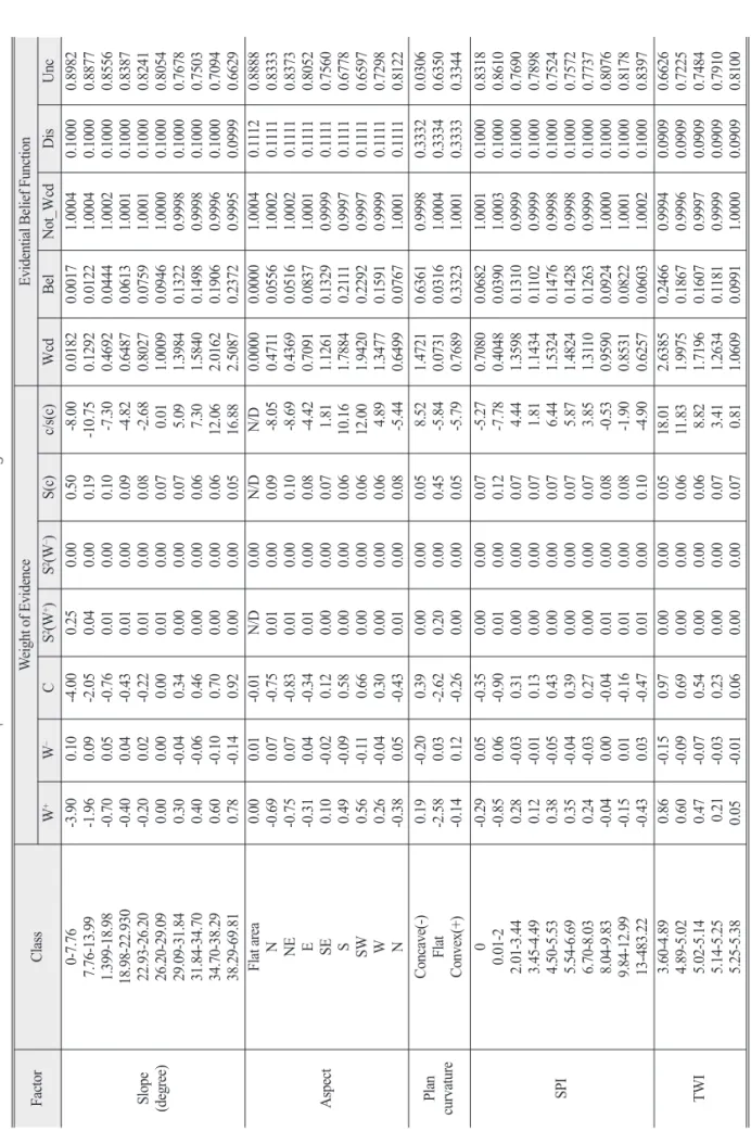
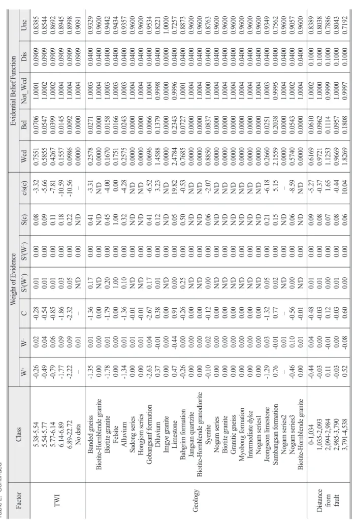
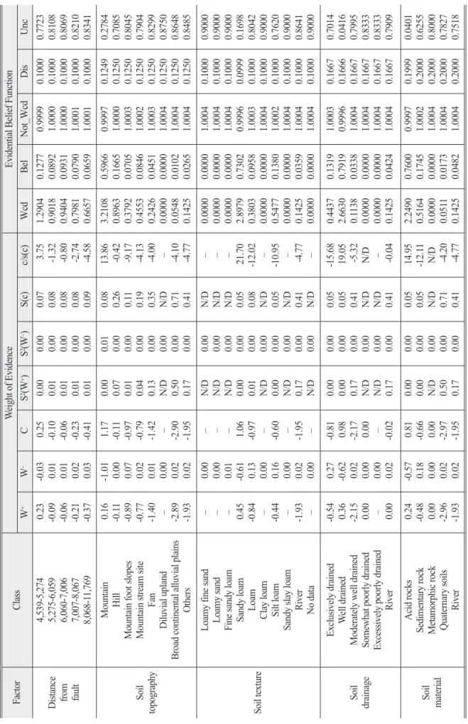
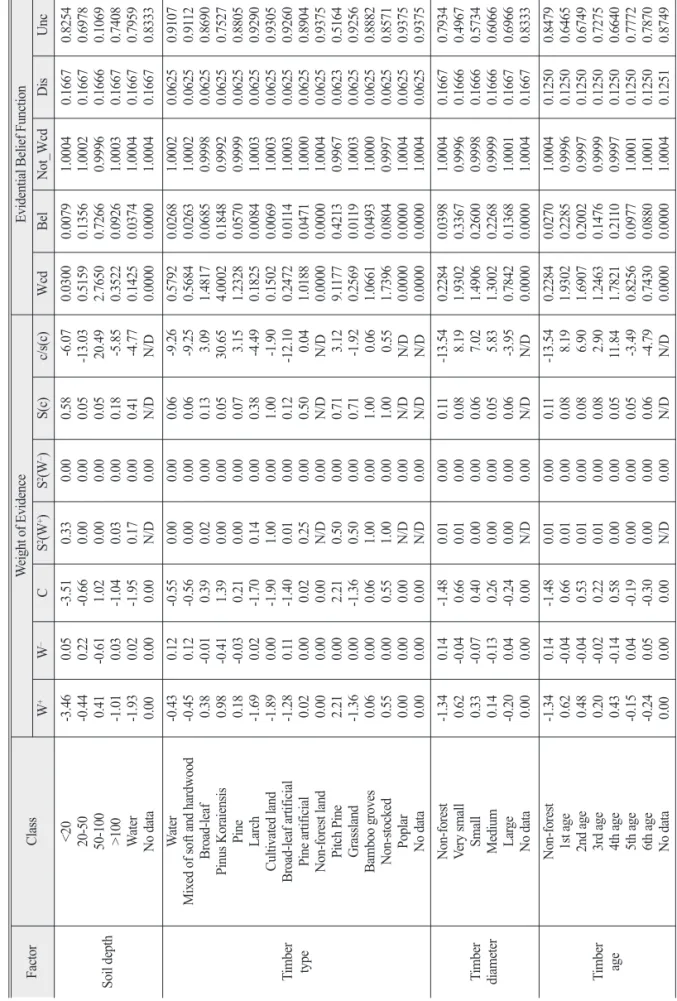
본 연구에서는 WOE, EBF, ANN 모델을 사용하여 연구지역의 각 단위 셀에 대한 산사태 취약성 값을 계 산하였다. 먼저 WOE 및 EBF 모델을 이용한 각 입력 요 인들과 훈련용 산사태 간의 공간적 상관관계는 Table 2 와 같다.

먼저 WOE의 계산 결과를 보면 입력자료 중 c/s(c)가 가장 큰 종류나 범위 값을 기준으로 W

와 W

를 구분하 게 된다 . 예를 들어 경사의 경우 c/s(c)가 가장 큰 범위는 38.29-69.81도 사이로 16.88값을 가지게 된다. 이럴 경우 38.29-69.81의 범위를 가지는 경사 분포는 W

값인 0.78을 가지고 되고 , 나머지 범위의 경사 분포는 W

값인 -0.14 의 값을 가지게 된다 . 나머지 입력 요인들의 경우도 같 은 방식으로 계산 및 해석이 된다 .

EBF 모델의 계산 결과를 보면 예를 들어, 경사도가 38°를 초과하는 경우, Belief과 DisBelief 값은 각각 0.2372 Fig. 3. Schematic relationships of evidential belief functions

(modified after Wright and Bonham-Carter, 1996;

Carranza et al., 2005).

Ta bl e 2. R ela tio ns hip s b et we en la nd sli de a nd e ac h fa ct or u sin g W O E an d EB F m od els Fa cto r Cl as s W eig ht of E vid en ce Ev ide nti al Be lie f F un cti on W

W

C S

(W

) S

(W

) S( c) c/s (c) W cd Be l No t_W cd Di s Un c Sl op e (d eg ree )

0- 7.7 6 7.7 6- 13 .99 1.3 99 -1 8.9 8 18 .98 -2 2.9 30 22 .93 -2 6.2 0 26 .20 -2 9.0 9 29 .09 -3 1.8 4 31 .84 -3 4.7 0 34 .70 -3 8.2 9 38 .29 -6 9.8 1

-3 .90 -1 .96 -0 .70 -0 .40 -0 .20 0.0 0 0.3 0 0.4 0 0.6 0 0.7 8

0.1 0 0.0 9 0.0 5 0.0 4 0.0 2 0.0 0 -0 .04 -0 .06 -0 .10 -0 .14

-4 .00 -2 .05 -0 .76 -0 .43 -0 .22 0.0 0 0.3 4 0.4 6 0.7 0 0.9 2

0.2 5 0.0 4 0.0 1 0.0 1 0.0 1 0.0 1 0.0 0 0.0 0 0.0 0 0.0 0

0.0 0 0.0 0 0.0 0 0.0 0 0.0 0 0.0 0 0.0 0 0.0 0 0.0 0 0.0 0

0.5 0 0.1 9 0.1 0 0.0 9 0.0 8 0.0 7 0.0 7 0.0 6 0.0 6 0.0 5

-8 .00 -1 0.7 5 -7 .30 -4 .82 -2.68 0.0 1 5.0 9 7.3 0 12 .06 16 .88

0.0 18 2 0.1 29 2 0.4 69 2 0.6 48 7 0.8 02 7 1.0 00 9 1.3 98 4 1.5 84 0 2.0 16 2 2.5 08 7

0.0 01 7 0.0 12 2 0.0 44 4 0.0 61 3 0.0 75 9 0.0 94 6 0.1 32 2 0.1 49 8 0.1 90 6 0.2 37 2

1.0 00 4 1.0 00 4 1.0 00 2 1.0 00 1 1.0 00 1 1.0 00 0 0.9 99 8 0.9 99 8 0.9 99 6 0.9 99 5

0.1 00 0 0.1 00 0 0.1 00 0 0.1 00 0 0.1 00 0 0.1 00 0 0.1 00 0 0.1 00 0 0.1 00 0 0.0 99 9

0.8 98 2 0.8 87 7 0.8 55 6 0.8 38 7 0.8 24 1 0.8 05 4 0.7 67 8 0.7 50 3 0.7 09 4 0.6 62 9 As pe ct

Fl at are a

N NE E SE S SW W N

0.0 0 -0 .69 -0 .75 -0 .31 0.1 0 0.4 9 0.5 6 0.2 6 -0 .38

0.0 1 0.0 7 0.0 7 0.0 4 -0 .02 -0 .09 -0 .11 -0 .04 0.0 5

-0 .01 -0 .75 -0 .83 -0 .34 0.1 2 0.5 8 0.6 6 0.3 0 -0 .43

N/ D 0.0 1 0.0 1 0.0 1 0.0 0 0.0 0 0.0 0 0.0 0 0.0 1

0.0 0 0.0 0 0.0 0 0.0 0 0.0 0 0.0 0 0.0 0 0.0 0 0.0 0

N/ D 0.0 9 0.1 0 0.0 8 0.0 7 0.0 6 0.0 6 0.0 6 0.0 8

N/ D -8 .05 -8 .69 -4.42 1.8 1 10 .16 12 .00 4.8 9 -5 .44

0.0 00 0 0.4 71 1 0.4 36 9 0.7 09 1 1.1 26 1 1.7 88 4 1.9 42 0 1.3 47 7 0.6 49 9

0.0 00 0 0.0 55 6 0.0 51 6 0.0 83 7 0.1 32 9 0.2 11 1 0.2 29 2 0.1 59 1 0.0 76 7

1.0 00 4 1.0 00 2 1.0 00 2 1.0 00 1 0.9 99 9 0.9 99 7 0.9 99 7 0.9 99 9 1.0 00 1

0.1 11 2 0.1 11 1 0.1 11 1 0.1 11 1 0.1 11 1 0.1 11 1 0.1 11 1 0.1 11 1 0.1 11 1

0.8 88 8 0.8 33 3 0.8 37 3 0.8 05 2 0.7 56 0 0.6 77 8 0.6 59 7 0.7 29 8 0.8 12 2 Pl an cu rv atu re Co nc av e(- ) Fl at Co nv ex (+ )

0.1 9 -2 .58 -0 .14

-0 .20 0.0 3 0.1 2

0.3 9 -2 .62 -0 .26

0.0 0 0.2 0 0.0 0

0.0 0 0.0 0 0.0 0

0.0 5 0.4 5 0.0 5

8.5 2 -5 .84 -5 .79

1.4 72 1 0.0 73 1 0.7 68 9

0.6 36 1 0.0 31 6 0.3 32 3

0.9 99 8 1.0 00 4 1.0 00 1

0.3 33 2 0.3 33 4 0.3 33 3

0.0 30 6 0.6 35 0 0.3 34 4 SP I

0 0.0 1- 2 2.0 1- 3.4 4 3.4 5- 4.4 9 4.5 0- 5.5 3 5.5 4- 6.6 9 6.7 0- 8.0 3 8.0 4- 9.8 3 9.8 4- 12 .99 13 -4 83 .22

-0 .29 -0 .85 0.2 8 0.1 2 0.3 8 0.3 5 0.2 4 -0 .04 -0 .15 -0 .43

0.0 5 0.0 6 -0 .03 -0 .01 -0 .05 -0 .04 -0 .03 0.0 0 0.0 1 0.0 3

-0 .35 -0 .90 0.3 1 0.1 3 0.4 3 0.3 9 0.2 7 -0 .04 -0 .16 -0 .47

0.0 0 0.0 1 0.0 0 0.0 0 0.0 0 0.0 0 0.0 0 0.0 1 0.0 1 0.0 1

0.0 0 0.0 0 0.0 0 0.0 0 0.0 0 0.0 0 0.0 0 0.0 0 0.0 0 0.0 0

0.0 7 0.1 2 0.0 7 0.0 7 0.0 7 0.0 7 0.0 7 0.0 8 0.0 8 0.1 0

-5 .27 -7 .78 4.4 4 1.8 1 6.4 4 5.8 7 3.8 5 -0 .53 -1 .90 -4 .90

0.7 08 0 0.4 04 8 1.3 59 8 1.1 43 4 1.5 32 4 1.4 82 4 1.3 11 0 0.9 59 0 0.8 53 1 0.6 25 7

0.0 68 2 0.0 39 0 0.1 31 0 0.1 10 2 0.1 47 6 0.1 42 8 0.1 26 3 0.0 92 4 0.0 82 2 0.0 60 3

1.0 00 1 1.0 00 3 0.9 99 9 0.9 99 9 0.9 99 8 0.9 99 8 0.9 99 9 1.0 00 0 1.0 00 1 1.0 00 2

0.1 00 0 0.1 00 0 0.1 00 0 0.1 00 0 0.1 00 0 0.1 00 0 0.1 00 0 0.1 00 0 0.1 00 0 0.1 00 0

0.8 31 8 0.8 61 0 0.7 69 0 0.7 89 8 0.7 52 4 0.7 57 2 0.7 73 7 0.8 07 6 0.8 17 8 0.8 39 7 TW I

3.6 0- 4.8 9 4.8 9- 5.0 2 5.0 2- 5.1 4 5.1 4- 5.2 5 5.2 5- 5.3 8

0.8 6 0.6 0 0.4 7 0.2 1 0.0 5

-0 .15 -0 .09 -0 .07 -0 .03 -0 .01

0.9 7 0.6 9 0.5 4 0.2 3 0.0 6

0.0 0 0.0 0 0.0 0 0.0 0 0.0 0

0.0 0 0.0 0 0.0 0 0.0 0 0.0 0

0.0 5 0.0 6 0.0 6 0.0 7 0.0 7

18 .01 11 .83 8.8 2 3.4 1 0.8 1

2.6 38 5 1.9 97 5 1.7 19 6 1.2 63 4 1.0 60 9

0.2 46 6 0.1 86 7 0.1 60 7 0.1 18 1 0.0 99 1

0.9 99 4 0.9 99 6 0.9 99 7 0.9 99 9 1.0 00 0

0.0 90 9 0.0 90 9 0.0 90 9 0.0 90 9 0.0 90 9

0.6 62 6 0.7 22 5 0.7 48 4 0.7 91 0 0.8 10 0

Ta bl e 2. C on tin ue d Fa cto r Cl as s W eig ht of E vid en ce Ev ide nti al Be lie f F un cti on W

W

C S

(W

) S

(W

) S( c) c/s (c) W cd Be l No t_W cd Di s Un c TW I

5.3 8- 5.5 4 5.5 4- 5.7 7 5.7 7- 6.1 4 6.1 4- 6.8 9 6.8 9- 22 .72 No da ta

-0 .26 -0 .49 -0 .79 -1 .77 -2 .22 –

0.0 2 0.0 4 0.0 6 0.0 9 0.0 9 0.0 1

-0 .28 -0 .54 -0 .85 -1 .86 -2 .32 –

0.0 1 0.0 1 0.0 1 0.0 3 0.0 5 N/ D

0.0 0 0.0 0 0.0 0 0.0 0 0.0 0 0.0 0

0.0 8 0.0 9 0.1 1 0.1 8 0.2 2 N/ D

-3 .32 -5 .66 -7 .81 -1 0.5 9 -1 0.5 6 –

0.7 55 1 0.5 85 5 0.4 26 7 0.1 55 7 0.0 98 6 0.0 00 0

0.0 70 6 0.0 54 7 0.0 39 9 0.0 14 5 0.0 09 2 0.0 00 0

1.0 00 1 1.0 00 2 1.0 00 2 1.0 00 4 1.0 00 4 1.0 00 4

0.0 90 9 0.0 90 9 0.0 90 9 0.0 90 9 0.0 90 9 0.0 90 9

0.8 38 5 0.8 54 4 0.8 69 2 0.8 94 5 0.8 99 8 0.9 09 1 Ge olo gy

Ba nd ed gn eis s Bi oti te- Ho rn ble nd e g ran ite Bi oti te gr an ite Fe lsi te Al luv ium Sa do ng se rie s Ho ng jom se rie s Go ba ng sa nf fo rm ati on Di luv ium Im gy e g ran ite Li me sto ne Ba bg rim fo rm ati on Ja ng sa n q ua rtz ite Bi oti te- Ho rn ble nd e g ran od ior ite Sy en ite No ga m se rie s Bi oti te gr an ite Gr an itic gn eis s M yo bo ng fo rm ati on In ter me dia te dy ke No ga m se rie s1 Je on gs eo n l im es ton e Sa mb an gs an fo rm ati on No ga m se rie s2 No ga m se rie s3 Bi oti te- Ho rn ble nd e g ran ite

-1 .35 0.0 0 -1 .78 0.0 0 -1 .34 0.0 0 0.0 0 -2 .63 0.3 7 0.0 0 0.4 7 -0 .26 0.0 0 0.0 0 -0 .10 0.0 0 0.0 0 0.0 0 0.0 0 0.0 0 0.0 0 -1 .29 0.7 6 – -0 .46 0.0 0

0.0 1 0.0 0 0.0 1 0.0 0 0.0 1 0.0 1 0.0 1 0.0 4 -0 .01 0.0 0 -0 .44 0.0 0 0.0 0 0.0 0 0.0 2 0.0 0 0.0 0 0.0 0 0.0 0 0.0 0 0.0 0 0.0 3 -0 .01 0.0 1 0.1 0 0.0 1

-1 .36 0.0 0 -1 .79 0.0 0 -1 .36 -0 .01 -0 .01 -2 .67 0.3 8 0.0 0 0.9 1 -0 .26 0.0 0 0.0 0 -0 .12 0.0 0 0.0 0 0.0 0 0.0 0 0.0 0 0.0 0 -1 .32 0.7 7 – -0 .56 -0 .01

0.1 7 N/ D 0.2 0 1.0 0 0.1 0 N/ D N/ D 0.1 7 0.0 1 N/ D 0.0 0 0.2 5 N/ D N/ D 0.0 0 N/ D N/ D N/ D N/ D N/ D N/ D 0.0 5 0.0 2 N/ D 0.0 0 N/ D

0.0 0 0.0 0 0.0 0 0.0 0 0.0 0 0.0 0 0.0 0 0.0 0 0.0 0 0.0 0 0.0 0 0.0 0 0.0 0 0.0 0 0.0 0 0.0 0 0.0 0 0.0 0 0.0 0 0.0 0 0.0 0 0.0 0 0.0 0 0.0 0 0.0 0 0.0 0

0.4 1 N/ D 0.4 5 1.0 0 0.3 2 N/ D N/ D 0.4 1 0.1 2 N/ D 0.0 5 0.5 0 N/ D N/ D 0.0 6 N/ D N/ D N/ D N/ D N/ D N/ D 0.2 1 0.1 5 N/ D 0.0 6 N/ D

-3 .31 N/ D -4 .00 0.0 0 -4 .28 N/ D N/ D -6 .52 3.2 3 N/ D 19 .82 -0.5 3 N/ D N/ D -2 .07 N/ D N/ D N/ D N/ D N/ D N/ D -6 .18 5.1 5

– -8.5 9 N/ D

0.2 57 8 0.0 00 0 0.1 67 0 0.1 75 1 0.2 57 5 0.0 00 0 0.0 00 0 0.0 69 6 1.4 58 8 0.0 00 0 2.4 78 4 0.7 68 5 0.0 00 0 0.0 00 0 0.8 85 0 0.0 00 0 0.0 00 0 0.0 00 0 0.0 00 0 0.0 00 0 0.0 00 0 0.2 66 0 2.1 55 9 0.0 00 0 0.5 74 0 0.0 00 0

0.0 27 1 0.0 00 0 0.0 15 8 0.0 16 6 0.0 24 3 0.0 00 0 0.0 00 0 0.0 06 6 0.1 37 9 0.0 00 0 0.2 34 3 0.0 72 7 0.0 00 0 0.0 00 0 0.0 83 7 0.0 00 0 0.0 00 0 0.0 00 0 0.0 00 0 0.0 00 0 0.0 00 0 0.0 25 1 0.2 03 8 0.0 00 0 0.0 54 3 0.0 00 0

1.0 00 3 1.0 00 4 1.0 00 3 1.0 00 3 1.0 00 3 1.0 00 4 1.0 00 4 1.0 00 4 0.9 99 8 0.0 00 0 0.9 99 6 1.0 00 1 1.0 00 4 1.0 00 4 1.0 00 0 1.0 00 4 1.0 00 4 1.0 00 4 1.0 00 4 1.0 00 4 1.0 00 4 1.0 00 3 0.9 99 5 1.0 00 4 1.0 00 2 1.0 00 4

0.0 40 0 0.0 40 0 0.0 40 0 0.0 40 0 0.0 40 0 0.0 40 0 0.0 40 0 0.0 40 0 0.0 40 0 0.0 00 0 0.0 40 0 0.0 40 0 0.0 40 0 0.0 40 0 0.0 40 0 0.0 40 0 0.0 40 0 0.0 40 0 0.0 40 0 0.0 40 0 0.0 40 0 0.0 40 0 0.0 40 0 0.0 40 0 0.0 40 0 0.0 40 0

0.9 32 9 0.9 60 0 0.9 44 2 0.9 43 4 0.9 35 7 0.9 60 0 0.9 60 0 0.9 53 4 0.8 22 1 1.0 00 0 0.7 25 7 0.8 87 3 0.9 60 0 0.9 60 0 0.8 76 3 0.9 60 0 0.9 60 0 0.9 60 0 0.9 60 0 0.9 60 0 0.9 60 0 0.9 34 9 0.7 56 2 0.9 60 0 0.9 05 7 0.9 60 0 Di sta nc e fro m fau lt

0- 1,0 34 1,0 35 -2 ,09 3 2,0 94 -2 ,98 4 2,9 85 -3 ,79 0 3,7 91 -4 ,53 8

-0 .44 -0 .03 0.1 1 -0 .03 0.5 2

0.0 4 0.0 0 -0 .01 0.0 0 -0 .08

-0 .48 -0 .03 0.1 2 -0 .03 0.6 0

0.0 1 0.0 1 0.0 0 0.0 1 0.0 0

0.0 0 0.0 0 0.0 0 0.0 0 0.0 0

0.0 9 0.0 8 0.0 7 0.0 8 0.0 6

-5 .27 -0 .37 1.6 5 -0 .44 10 .04

0.6 16 9 0.9 72 1 1.1 25 3 0.9 66 9 1.8 26 9

0.0 61 0 0.0 96 2 0.1 11 4 0.0 95 7 0.1 80 8

1.0 00 2 1.0 00 0 0.9 99 9 1.0 00 0 0.9 99 7

0.1 00 0 0.1 00 0 0.1 00 0 0.1 00 0 0.1 00 0

0.8 38 9 0.8 03 8 0.7 88 6 0.8 04 3 0.7 19 2

Ta bl e 2. C on tin ue d Fa cto r Cl as s W eig ht of E vid en ce Ev ide nti al Be lie f F un cti on W

W

C S

(W

) S

(W

) S( c) c/s (c) W cd Be l No t_W cd Di s Un c Di sta nc e fro m fau lt

4,5 39 -5 ,27 4 5,2 75 -6 ,05 9 6,0 60 -7 ,00 6 7,0 07 -8 ,06 7 8,0 68 -11 ,76 9

0.2 3 -0 .09 -0 .06 -0 .21 -0 .37

-0 .03 0.0 1 0.0 1 0.0 2 0.0 3

0.2 5 -0 .10 -0 .06 -0 .23 -0 .41

0.0 0 0.0 1 0.0 1 0.0 1 0.0 1

0.0 0 0.0 0 0.0 0 0.0 0 0.0 0

0.0 7 0.0 8 0.0 8 0.0 8 0.0 9

3.7 5 -1 .32 -0 .80 -2 .74 -4 .58

1.2 90 4 0.9 01 8 0.9 40 4 0.7 98 1 0.6 65 7

0.1 27 7 0.0 89 2 0.0 93 1 0.0 79 0 0.0 65 9

0.9 99 9 1.0 00 0 1.0 00 0 1.0 00 1 1.0 00 1

0.1 00 0 0.1 00 0 0.1 00 0 0.1 00 0 0.1 00 0

0.7 72 3 0.8 10 8 0.8 06 9 0.8 21 0 0.8 34 1 So il top og rap hy

M ou nta in Hi ll M ou nta in fo ot slo pe s M ou nta in str ea m sit e Fa n Di luv ial up lan d Br oa d c on tin en tal al luv ial pl ain s Ot he rs

0.1 6 -0 .11 -0 .89 -0 .77 -1.40 – -2.8 9 -1 .93

-1 .01 0.0 0 0.0 7 0.0 2 0.0 1 0.0 0 0.0 2 0.0 2

1.1 7 -0 .11 -0 .97 -0 .79 -1.42 – -2.9 0 -1 .95

0.0 0 0.0 7 0.0 1 0.0 4 0.1 3 N/ D 0.5 0 0.1 7

0.0 1 0.0 0 0.0 0 0.0 0 0.0 0 0.0 0 0.0 0 0.0 0

0.0 8 0.2 6 0.1 1 0.1 9 0.3 5 N/ D 0.7 1 0.4 1

13 .86 -0.4 2 -9 .17 -4 .13 -4.00 – -4.1 0 -4 .77

3.2 10 8 0.8 96 3 0.3 79 2 0.4 55 3 0.2 42 6 0.0 00 0 0.0 54 8 0.1 42 5

0.5 96 6 0.1 66 5 0.0 70 5 0.0 84 6 0.0 45 1 0.0 00 0 0.0 10 2 0.0 26 5

0.9 99 7 1.0 00 0 1.0 00 3 1.0 00 2 1.0 00 3 1.0 00 4 1.0 00 4 1.0 00 4

0.1 24 9 0.1 25 0 0.1 25 0 0.1 25 0 0.1 25 0 0.1 25 0 0.1 25 0 0.1 25 0

0.2 78 4 0.7 08 5 0.8 04 5 0.7 90 4 0.8 29 9 0.8 75 0 0.8 64 8 0.8 48 5 So il t ex tur e

Lo am y f ine sa nd Lo am y s an d Fi ne sa nd y l oa m Sa nd y l oa m Lo am Cl ay lo am Si lt l oa m Sa nd y s lay lo am Ri ve r No da ta

– – – 0.4 5

-0.84 – -0.4 4 – -1 .93 –

0.0 0 0.0 0 0.0 1 -0 .61 0.1 3 0.0 0 0.1 6 0.0 0 0.0 2 0.0 0

– – – 1.0 6

-0.97 – -0.6 0 – -1 .95 –

N/ D N/ D N/ D 0.0 0 0.0 1 N/ D 0.0 0 N/ D 0.1 7 N/ D

0.0 0 0.0 0 0.0 0 0.0 0 0.0 0 0.0 0 0.0 0 0.0 0 0.0 0 0.0 0

N/ D N/ D N/ D 0.0 5 0.0 8 N/ D 0.0 5 N/ D 0.4 1 N/ D

– – – 21. 70 -1 2.0 2 – -1 0.9 5

– -4.7 7 –

0.0 00 0 0.0 00 0 0.0 00 0 2.8 97 9 0.3 80 3 0.0 00 0 0.5 47 7 0.0 00 0 0.1 42 5 0.0 00 0

0.0 00 0 0.0 00 0 0.0 00 0 0.7 30 2 0.0 95 8 0.0 00 0 0.1 38 0 0.0 00 0 0.0 35 9 0.0 00 0

1.0 00 4 1.0 00 4 1.0 00 4 0.9 99 6 1.0 00 3 1.0 00 4 1.0 00 2 1.0 00 4 1.0 00 4 1.0 00 4

0.1 00 0 0.1 00 0 0.1 00 0 0.0 99 9 0.1 00 0 0.1 00 0 0.1 00 0 0.1 00 0 0.1 00 0 0.1 00 0

0.9 00 0 0.9 00 0 0.9 00 0 0.1 69 8 0.8 04 2 0.9 00 0 0.7 62 0 0.9 00 0 0.8 64 1 0.9 00 0 So il dr ain ag e

Ex clu siv ely dr ain ed W ell dr ain ed M od era tel y w ell dr ain ed So me wh at po or ly dr ain ed Ex ce ssi ve ly po or ly dr ain ed Ri ve r

-0 .54 0.3 6 -2 .15 0.0 0 – 0.0 0

0.2 7 -0 .62 0.0 2 0.0 0 0.0 0 0.0 2

-0 .81 0.9 8 -2 .17 0.0 0 – -0 .02

0.0 0 0.0 0 0.1 7 N/ D N/ D 0.1 7

0.0 0 0.0 0 0.0 0 0.0 0 0.0 0 0.0 0

0.0 5 0.0 5 0.4 1 N/ D N/ D 0.4 1

-1 5.6 8 19 .05 -5.3 2

N/D – -0.0 4

0.4 43 7 2.6 63 0 0.1 13 8 0.0 00 0 0.0 00 0 0.1 42 5

0.1 31 9 0.7 91 9 0.0 33 8 0.0 00 0 0.0 00 0 0.0 42 4

1.0 00 3 0.9 99 6 1.0 00 4 1.0 00 4 1.0 00 4 1.0 00 4

0.1 66 7 0.1 66 6 0.1 66 7 0.1 66 7 0.1 66 7 0.1 66 7

0.7 01 4 0.0 41 6 0.7 99 5 0.8 33 3 0.8 33 3 0.7 90 9 So il ma ter ial

Ac id ro ck s Se dim en tar y r oc k M eta mo rp hic ro ck Qu ate rn ary so ils Ri ve r

0.2 4 -0 .48 0.0 0 -2 .96 -1 .93

-0 .57 0.1 8 0.0 0 0.0 2 0.0 2

0.8 1 -0 .66 0.0 0 -2 .97 -1 .95

0.0 0 0.0 0 N/ D 0.5 0 0.1 7

0.0 0 0.0 0 0.0 0 0.0 0 0.0 0

0.0 5 0.0 5 N/ D 0.7 1 0.4 1

14 .95 -1 2.1 1 N/ D -4 .20 -4 .77

2.2 49 0 0.5 16 4 0.0 00 0 0.0 51 1 0.1 42 5

0.7 60 0 0.1 74 5 0.0 00 0 0.0 17 3 0.0 48 2

0.9 99 7 1.0 00 2 1.0 00 4 1.0 00 4 1.0 00 4

0.1 99 9 0.2 00 0 0.2 00 0 0.2 00 0 0.2 00 0

0.0 40 1 0.6 25 5 0.8 00 0 0.7 82 7 0.7 51 8

Ta bl e 2. C on tin ue d Fa cto r Cl as s W eig ht of E vid en ce Ev ide nti al Be lie f F un cti on W

W

C S

(W

) S

(W

) S( c) c/s (c) W cd Be l No t_W cd Di s Un c So il d ep th

<2 0 20 -5 0 50 -1 00 >1 00 W ate r No da ta

-3 .46 -0 .44 0.4 1 -1 .01 -1 .93 0.0 0

0.0 5 0.2 2 -0 .61 0.0 3 0.0 2 0.0 0

-3 .51 -0 .66 1.0 2 -1 .04 -1 .95 0.0 0

0.3 3 0.0 0 0.0 0 0.0 3 0.1 7 N/ D

0.0 0 0.0 0 0.0 0 0.0 0 0.0 0 0.0 0

0.5 8 0.0 5 0.0 5 0.1 8 0.4 1 N/ D

-6 .07 -1 3.0 3 20 .49 -5.8 5 -4 .77 N/ D

0.0 30 0 0.5 15 9 2.7 65 0 0.3 52 2 0.1 42 5 0.0 00 0

0.0 07 9 0.1 35 6 0.7 26 6 0.0 92 6 0.0 37 4 0.0 00 0

1.0 00 4 1.0 00 2 0.9 99 6 1.0 00 3 1.0 00 4 1.0 00 4

0.1 66 7 0.1 66 7 0.1 66 6 0.1 66 7 0.1 66 7 0.1 66 7

0.8 25 4 0.6 97 8 0.1 06 9 0.7 40 8 0.7 95 9 0.8 33 3 Ti mb er typ e

W ate r M ixe d o f s of t a nd ha rd wo od Br oa d- lea f Pi nu s K or aie ns is Pi ne La rch Cu ltiv ate d l an d Br oa d- lea f a rti fic ial Pi ne ar tif ici al No n- fo res t la nd Pi tch Pi ne Gr as sla nd Ba mb oo gr ov es No n- sto ck ed Po pla r No da ta

-0 .43 -0 .45 0.3 8 0.9 8 0.1 8 -1 .69 -1 .89 -1 .28 0.0 2 0.0 0 2.2 1 -1 .36 0.0 6 0.5 5 0.0 0 0.0 0

0.1 2 0.1 2 -0 .01 -0 .41 -0 .03 0.0 2 0.0 0 0.1 1 0.0 0 0.0 0 0.0 0 0.0 0 0.0 0 0.0 0 0.0 0 0.0 0

-0 .55 -0 .56 0.3 9 1.3 9 0.2 1 -1 .70 -1 .90 -1 .40 0.0 2 0.0 0 2.2 1 -1 .36 0.0 6 0.5 5 0.0 0 0.0 0

0.0 0 0.0 0 0.0 2 0.0 0 0.0 0 0.1 4 1.0 0 0.0 1 0.2 5 N/ D 0.5 0 0.5 0 1.0 0 1.0 0 N/ D N/ D

0.0 0 0.0 0 0.0 0 0.0 0 0.0 0 0.0 0 0.0 0 0.0 0 0.0 0 0.0 0 0.0 0 0.0 0 0.0 0 0.0 0 0.0 0 0.0 0

0.0 6 0.0 6 0.1 3 0.0 5 0.0 7 0.3 8 1.0 0 0.1 2 0.5 0 N/ D 0.7 1 0.7 1 1.0 0 1.0 0 N/ D N/ D

-9 .26 -9 .25 3.0 9 30 .65 3.1 5 -4 .49 -1 .90 -1 2.1 0 0.0 4 N/ D 3.1 2 -1 .92 0.0 6 0.5 5 N/ D N/ D

0.5 79 2 0.5 68 4 1.4 81 7 4.0 00 2 1.2 32 8 0.1 82 5 0.1 50 2 0.2 47 2 1.0 18 8 0.0 00 0 9.1 17 7 0.2 56 9 1.0 66 1 1.7 39 6 0.0 00 0 0.0 00 0

0.0 26 8 0.0 26 3 0.0 68 5 0.1 84 8 0.0 57 0 0.0 08 4 0.0 06 9 0.0 11 4 0.0 47 1 0.0 00 0 0.4 21 3 0.0 11 9 0.0 49 3 0.0 80 4 0.0 00 0 0.0 00 0

1.0 00 2 1.0 00 2 0.9 99 8 0.9 99 2 0.9 99 9 1.0 00 3 1.0 00 3 1.0 00 3 1.0 00 0 1.0 00 4 0.9 96 7 1.0 00 3 1.0 00 0 0.9 99 7 1.0 00 4 1.0 00 4

0.0 62 5 0.0 62 5 0.0 62 5 0.0 62 5 0.0 62 5 0.0 62 5 0.0 62 5 0.0 62 5 0.0 62 5 0.0 62 5 0.0 62 3 0.0 62 5 0.0 62 5 0.0 62 5 0.0 62 5 0.0 62 5

0.9 10 7 0.9 11 2 0.8 69 0 0.7 52 7 0.8 80 5 0.9 29 0 0.9 30 5 0.9 26 0 0.8 90 4 0.9 37 5 0.5 16 4 0.9 25 6 0.8 88 2 0.8 57 1 0.9 37 5 0.9 37 5 Ti mb er dia me ter

No n- fo res t Ve ry sm all Sm all M ed ium La rg e No da ta

-1 .34 0.6 2 0.3 3 0.1 4 -0 .20 0.0 0

0.1 4 -0 .04 -0 .07 -0 .13 0.0 4 0.0 0

-1 .48 0.6 6 0.4 0 0.2 6 -0 .24 0.0 0

0.0 1 0.0 1 0.0 0 0.0 0 0.0 0 N/ D

0.0 0 0.0 0 0.0 0 0.0 0 0.0 0 0.0 0

0.1 1 0.0 8 0.0 6 0.0 5 0.0 6 N/ D

-1 3.5 4 8.1 9 7.0 2 5.8 3 -3 .95 N/ D

0.2 28 4 1.9 30 2 1.4 90 6 1.3 00 2 0.7 84 2 0.0 00 0

0.0 39 8 0.3 36 7 0.2 60 0 0.2 26 8 0.1 36 8 0.0 00 0

1.0 00 4 0.9 99 6 0.9 99 8 0.9 99 9 1.0 00 1 1.0 00 4

0.1 66 7 0.1 66 6 0.1 66 6 0.1 66 6 0.1 66 7 0.1 66 7

0.7 93 4 0.4 96 7 0.5 73 4 0.6 06 6 0.6 96 6 0.8 33 3 Ti mb er ag e

No n- fo res t 1s t a ge 2n d a ge 3r d a ge 4th ag e 5th ag e 6th ag e No da ta

-1 .34 0.6 2 0.4 8 0.2 0 0.4 3 -0 .15 -0 .24 0.0 0

0.1 4 -0 .04 -0 .04 -0 .02 -0 .14 0.0 4 0.0 5 0.0 0

-1 .48 0.6 6 0.5 3 0.2 2 0.5 8 -0 .19 -0 .30 0.0 0

0.0 1 0.0 1 0.0 1 0.0 1 0.0 0 0.0 0 0.0 0 N/ D

0.0 0 0.0 0 0.0 0 0.0 0 0.0 0 0.0 0 0.0 0 0.0 0

0.1 1 0.0 8 0.0 8 0.0 8 0.0 5 0.0 5 0.0 6 N/ D

-1 3.5 4 8.1 9 6.9 0 2.9 0 11 .84 -3.4 9 -4 .79 N/ D

0.2 28 4 1.9 30 2 1.6 90 7 1.2 46 3 1.7 82 1 0.8 25 6 0.7 43 0 0.0 00 0

0.0 27 0 0.2 28 5 0.2 00 2 0.1 47 6 0.2 11 0 0.0 97 7 0.0 88 0 0.0 00 0

1.0 00 4 0.9 99 6 0.9 99 7 0.9 99 9 0.9 99 7 1.0 00 1 1.0 00 1 1.0 00 4

0.1 25 0 0.1 25 0 0.1 25 0 0.1 25 0 0.1 25 0 0.1 25 0 0.1 25 0 0.1 25 1

0.8 47 9 0.6 46 5 0.6 74 9 0.7 27 5 0.6 64 0 0.7 77 2 0.7 87 0 0.8 74 9

Ta bl e 2. C on tin ue d Fa cto r Cl as s W eig ht of E vid en ce Ev ide nti al Be lie f F un cti on W

W

C S

(W

) S

(W

) S( c) c/s (c) W cd Be l No t_W cd Di s Un c Ti mb er de ns ity

No n- fo res t Lo os e M od era te De ns e

0.0 1 0.2 2 1.2 3 -0 .50

-0 .01 -0 .09 -0 .02 0.1 0

0.0 2 0.3 1 1.2 4 -0 .61

0.0 0 0.0 0 0.0 2 0.0 0

0.0 0 0.0 0 0.0 0 0.0 0

0.0 5 0.0 5 0.1 6 0.0 7

0.5 4 6.5 2 7.9 7 -9 .09

1.0 24 4 1.3 68 9 3.4 69 5 0.5 45 2

0.1 59 9 0.2 13 6 0.5 41 4 0.0 85 1

1.0 00 0 0.9 99 9 0.9 99 0 1.0 00 2

0.2 50 1 0.2 50 0 0.2 49 8 0.2 50 1

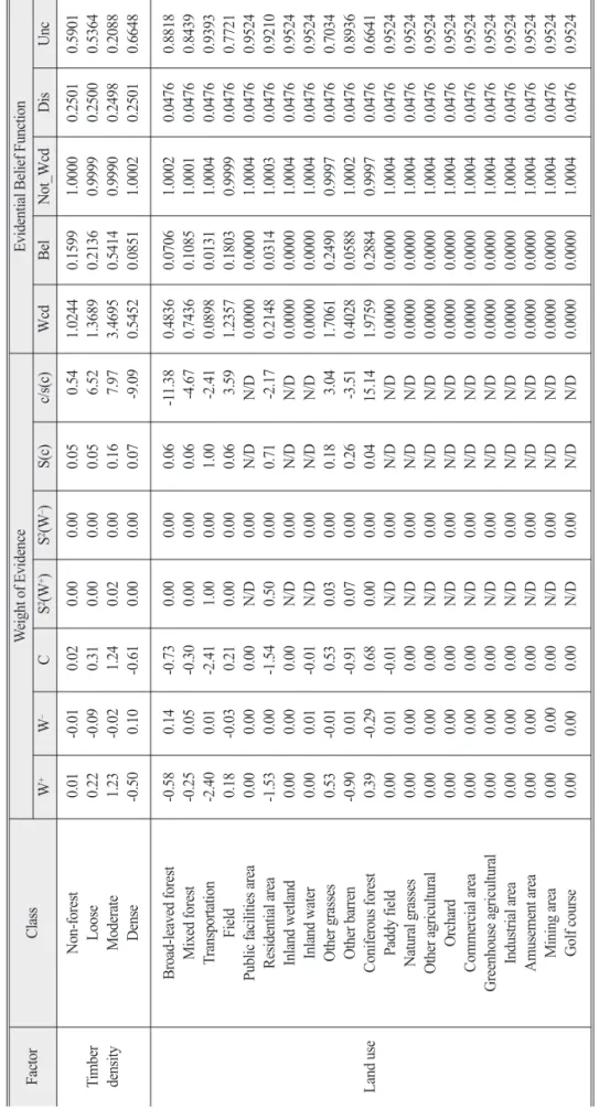
0.5 90 1 0.5 36 4 0.2 08 8 0.6 64 8 La nd us e

Br oa d- lea ve d f or es t M ixe d f or es t Tr an sp or tat ion Fi eld Pu bli c f ac ilit ies ar ea Re sid en tia l a rea In lan d w etl an d In lan d w ate r Ot he r g ras se s Ot he r b arr en Co nif ero us fo res t Pa dd y f iel d Na tur al gr as se s Ot he r a gr icu ltu ral Or ch ard Co mm erc ial ar ea Gr ee nh ou se ag ric ult ur al In du str ial ar ea Am us em en t a rea M ini ng ar ea Go lf co ur se

-0 .58 -0 .25 -2 .40 0.1 8 0.0 0 -1 .53 0.0 0 0.0 0 0.5 3 -0 .90 0.3 9 0.0 0 0.0 0 0.0 0 0.0 0 0.0 0 0.0 0 0.0 0 0.0 0 0.0 0 0.0 0

0.1 4 0.0 5 0.0 1 -0 .03 0.0 0 0.0 0 0.0 0 0.0 1 -0 .01 0.0 1 -0 .29 0.0 1 0.0 0 0.0 0 0.0 0 0.0 0 0.0 0 0.0 0 0.0 0 0.0 0 0.0 0

-0 .73 -0 .30 -2 .41 0.2 1 0.0 0 -1 .54 0.0 0 -0 .01 0.5 3 -0 .91 0.6 8 -0 .01 0.0 0 0.0 0 0.0 0 0.0 0 0.0 0 0.0 0 0.0 0 0.0 0 0.0 0

0.0 0 0.0 0 1.0 0 0.0 0 N/ D 0.5 0 N/ D N/ D 0.0 3 0.0 7 0.0 0 N/ D N/ D N/ D N/ D N/ D N/ D N/ D N/ D N/ D N/ D

0.0 0 0.0 0 0.0 0 0.0 0 0.0 0 0.0 0 0.0 0 0.0 0 0.0 0 0.0 0 0.0 0 0.0 0 0.0 0 0.0 0 0.0 0 0.0 0 0.0 0 0.0 0 0.0 0 0.0 0 0.0 0

0.0 6 0.0 6 1.0 0 0.0 6 N/ D 0.7 1 N/ D N/ D 0.1 8 0.2 6 0.0 4 N/ D N/ D N/ D N/ D N/ D N/ D N/ D N/ D N/ D N/ D

-11 .38 -4 .67 -2 .41 3.5 9 N/ D -2 .17 N/ D N/ D 3.0 4 -3 .51 15 .14 N/ D N/ D N/ D N/ D N/ D N/ D N/ D N/ D N/ D N/ D

0.4 83 6 0.7 43 6 0.0 89 8 1.2 35 7 0.0 00 0 0.2 14 8 0.0 00 0 0.0 00 0 1.7 06 1 0.4 02 8 1.9 75 9 0.0 00 0 0.0 00 0 0.0 00 0 0.0 00 0 0.0 00 0 0.0 00 0 0.0 00 0 0.0 00 0 0.0 00 0 0.0 00 0

0.0 70 6 0.1 08 5 0.0 13 1 0.1 80 3 0.0 00 0 0.0 31 4 0.0 00 0 0.0 00 0 0.2 49 0 0.0 58 8 0.2 88 4 0.0 00 0 0.0 00 0 0.0 00 0 0.0 00 0 0.0 00 0 0.0 00 0 0.0 00 0 0.0 00 0 0.0 00 0 0.0 00 0

1.0 00 2 1.0 00 1 1.0 00 4 0.9 99 9 1.0 00 4 1.0 00 3 1.0 00 4 1.0 00 4 0.9 99 7 1.0 00 2 0.9 99 7 1.0 00 4 1.0 00 4 1.0 00 4 1.0 00 4 1.0 00 4 1.0 00 4 1.0 00 4 1.0 00 4 1.0 00 4 1.0 00 4

0.0 47 6 0.0 47 6 0.0 47 6 0.0 47 6 0.0 47 6 0.0 47 6 0.0 47 6 0.0 47 6 0.0 47 6 0.0 47 6 0.0 47 6 0.0 47 6 0.0 47 6 0.0 47 6 0.0 47 6 0.0 47 6 0.0 47 6 0.0 47 6 0.0 47 6 0.0 47 6 0.0 47 6

0.8 81 8 0.8 43 9 0.9 39 3 0.7 72 1 0.9 52 4 0.9 21 0 0.9 52 4 0.9 52 4 0.7 03 4 0.8 93 6 0.6 64 1 0.9 52 4 0.9 52 4 0.9 52 4 0.9 52 4 0.9 52 4 0.9 52 4 0.9 52 4 0.9 52 4 0.9 52 4 0.9 52 4

과 0.0999로 산사태가 발생할 확률이 가장 높았으며, 경 사면의 경우 , 가장 높은 값은 남서쪽과 남쪽(각각 0.2292 과 0.2111)에 분포하며, 이들 범주는 산사태 발생과 양의 공간적 연관성이 있음을 보여 주었다 . 평면 곡률의 경 우 오목한 모양 (0.6361)에 대한 높은 Belief 값을 갖는다.

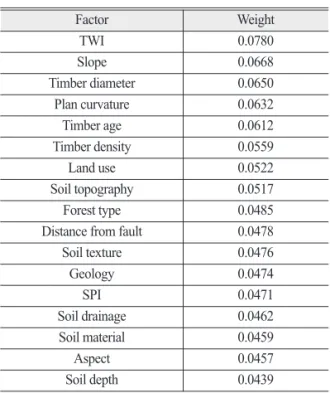
ANN의 경우 훈련 후, 가중치가 Table 3과 같이 결정 되었다 . 결과를 보면 TWI, 경사도, 임상경급, 곡률, 임상 영급 등이 가중치가 0.060 이상으로 높게 나왔고, 토양 두께, 경사방향, 토양모재, 토양배수, SPI 등이 낮게 나 왔다.

본 연구에서는 이러한 WOE, EBF, ANN 모델의 계 산 결과를 이용하여 산사태 취약성도를 작성하였다 . WOE 모델의 경우는 공식 (5)와 같이 각 입력 요인들은 W

와 W

값으로 2등분한 후 모든 입력 요인들의 W

와 W

값을 중첩분석을 통해 더하여 산사태 취약성 지수 를 계산하였다 . EBF 모델의 경우도 마찬가지로 공식 (11)과 같이 모든 입력 요인들의 belief값을 중첩분석을 통해 모두 더하여 산사태 취약성 지수를 계산하였다.

ANN 모델의 경우 산사태 취약성 지수값이 출력 레이어 로 0에서 1사이의 값을 가지도록 계산되었다. 이렇게 계 산된 산사태 취약성 지수는 ArcGIS에서 재분류를 통해 쉽게 시각적으로 해석할 수 있도록 5단계 즉 매우 높음, 높음 , 중간, 낮음, 매우 낮음으로 분류되었고, 각 분류는

전체 면적의 20%씩을 차지하도록 분류하였다(Fig. 4).

산사태 취약성도는 향후 산사태 발생에 위험 지역을 효과적으로 예측해야 하며, 미래에 발생할 새로운 산사 태 위치를 사용하여 이를 검증할 수 있다 . 산사태 위치 는 WOE, EBF, ANN 모델을 이용하여 산사태 취약성을 분석하는 훈련용 (50%)과 예측된 취약성도를 확인하는 검증용(50%)로 무작위로 나뉘었다. 산사태 취약성도의 정확도 분석 결과는 훈련에 사용되지 않는 알려진 산사 태 위치 (검증용)를 사용하여 검증되었다. 검증은 검증 용 산사태 위치와 산사태 취약성도를 비교함으로써 수 행되었다. 비율곡선(Lee and Sambath, 2006)을 작성하고 그 비율곡선 아래의 면적을 계산하였고 (Fig. 5), 그 비율 곡선과 비율곡선 아래의 면적은 모델과 입력 요인이 산 Table 3. Weight value for each factor

Factor Weight

TWI 0.0780

Slope 0.0668

Timber diameter 0.0650 Plan curvature 0.0632 Timber age 0.0612 Timber density 0.0559

Land use 0.0522

Soil topography 0.0517 Forest type 0.0485 Distance from fault 0.0478 Soil texture 0.0476

Geology 0.0474

SPI 0.0471

Soil drainage 0.0462 Soil material 0.0459

Aspect 0.0457

Soil depth 0.0439

Fig. 4. Landslide susceptibility maps using WOE, EBF and ANN.

(a) WOE

(b) EBF

(c) ANN

사태를 얼마나 잘 예측하는지를 설명한다 (Lee, 2005). 그 리고 곡선 아래의 영역은 예측 정확도를 정략적으로 평 가할 수 있다. 곡선은 취약성지수 순위의 면적 범위와 관련하여 산사태 누적을 보여준다(Fig. 5). X 축은 영역 의 누적 백분율을 나타내며 , 취약성지수 값의 최고 값 에서 최저값까지 정렬된다 . Y 축에서 산사태 누적 백분 율이 표시된다 . 예를 들어, 산사태 민감도 지수의 20%

를 넘는 지수 순위는 WOE, EBF, ANN 모델에 의해 모 든 산사태의 53%, 56% 및 44%를 설명할 수 있다(Fig. 5).

이러한 비율곡선 아래의 면적을 계산하여 각 모델들의 예측 정확도는 WOE, EBF, ANN 모델이 각각 74.73%, 75.03%, 및 70.87%로 계산되어 전체적으로 70% 이상을 값을 나타냈다 . 이 모델 중 EBF 모델이 가장 높은 예측 정확도를 나타냈다.

5. 토론 및 결론

본 연구에서는 WOE, EBF, ANN 모델과 각종 환경 공간정보를 사용하여 평창 지역의 산사태 취약성을 분 석하고 이를 도면으로 작성하였다 . 또한 본 취약성도의

예측 능력을 정량적으로 검증하였고 , 그 결과는 WOE 모델의 경우는 74.73%, EBF 모델의 경우는 75.03%, ANN 모델의 경우는 70.87%로 나타났다. 이러한 결과 로 볼 때 , 본 연구지역에서는 모든 모델이 70% 이상의 예측 능력을 보여주었으며 , 그중 EBF 모델이 가장 높은 예측 능력을 나타내었다 .

산사태 취약성도(Fig. 4)를 보면 확률 모델인 WOE 및 EBF 모델은 비슷한 공간 분포를 보였으나, ANN 모델 의 경우 위의 모델들과는 다른 공간분포를 보였다. 이는 훈련 자료에 따라 결과가 달라지는 ANN 모델의 한계를 보여주는 것으로, ANN 모델에서 훈련 자료 선택에 따 라 그 결과가 달라지는 것에 대한 연구가 필요하다 .

WOE 모델의 장점은 입력자료의 불확실성을 어느 정도 극복할 수 있다는 것이다 . 입력자료를 단순히 2가 지 분류 즉 , 우호적과 비우호적인 구분으로 분류하여 단 순화함으로써 , 입력자료가 부정확할 경우, 그 부정확성 을 어느 정도 극복하여 분석을 할 수 있는 장점이 있다 . 따라서 본 모델은 부정확한 자료 즉 지하공간 자료가 많 이 사용되는 광물 잠재성 지도 작성 등의 분야에 유용 하게 사용되어 왔다. EBF 모델의 장점은 다른 공간 데 이터 통합 모델과 달리 신념 , 불신, 불확실성 및 타당성 등 일련의 질량 기능을 지원한다는 점이다. 따라서 결 과는 불확실성의 정도를 모델링함으로써 산사태 발생 과 다중 공간 데이터 층 사이의 정량적 관계를 적절히 나타낼 수 있다 (Park, 2011). EBF 모델 또한 광물 잠재성 지도 작성 (Moon, 1989; An et al., 1992)에 대한 지식 기반 접근법에 적용되어왔다 . ANN 모델의 경우 입력 자료 의 통계적인 한계를 극복할 수 있고 , 각 요인의 가중치 를 정량적으로 계산할 수 있다는 장점이 있다. 또한 복 잡한 문제 및 복잡한 자료에 대해서도 입력자료를 훈련 시킴으로써 쉽게 해결할 수도 있다는 장점이 있다.

본 연구에서 제안된 WOE, EBF, ANN 모델과 산사 태 취약성도는 이전에 산사태가 발생하지 않은 지역의 산사태를 예측하는 데 사용될 수 있다 . 결국 이러한 취 약성도는 산사태 위험 감소를 촉진하고 , 토지 이용 정 책 및 개발을 위한 기초자료 역할을 할 수 있으며 , 궁극 적으로 산사태 재해 예방을 위한 시간과 비용을 절약할 수 있다 . 향후 보다 많은 지역에서 산사태 취약성도 작 성 방법을 적용하여 산사태 위험 예측을 위한 유용한 분 Fig. 5. Cumulative frequency diagram showing the landslide

susceptibility index rank (x-axis) occurring in the cumulative percent of landslide locations (y-axis).

From the validation of the landslide susceptibility

maps, WOE, EBF and ANN approaches the produced

AUC values of accuracy of 74.73%, 75.03% and

70.87% for each.

석 도구로 사용될 수 있는 좀 더 일반화된 모델을 이끌 어 내야 한다.

사 사

본 연구는 한국지질자원연구원 주요사업의 일환으 로 수행되었습니다 .

References

Althuwaynee, O.F., B. Pradhan, H.J. Park, and J.H.

Lee, 2014a. A novel ensemble bivariate statistical evidential belief function with knowledge-based analytical hierarchy process and multivariate statistical logistic regression for landslide susceptibility mapping, Catena, 114: 21-36.

Althuwaynee, O.F., B. Pradhan, H.J. Park, and J.H.

Lee, 2014b. A novel ensemble decision tree-based CHi-squared Automatic Interaction Detection (CHAID) and multivariate logistic regression models in landslide susceptibility mapping,

An, P., W. M. Moon, and G. F. Bonham-Carter, 1992.

On knowledge based approach to integrating remote sensing, geophysical and geological information, Proc. of International Geoscience

Clear Lake Area Houston, May 26-29, vol. 1, pp. 34-38.

Anbalagan, R., 1992. Landslide susceptibility evaluation and zonation mapping in mountainous terrain,

Bonham-Carter, G. F., 1994. Geographic Information

Pergamon Press, Oxford, UK.

Bonham-Carter, G.F., F.P. Agterberg, and D.F. Wright, 1988. Integration of geological datasets for gold exploration in Nova Scotia, Photogrammetic

Engineering and Remote Sensing, 54(11): 1585-

1592.

Bui, D.T., B. Pradhan, I. Revhaug, D.B. Nguyen, H.V.

Pham, and Q.N. Bui, 2015. A novel hybrid evidential belief function-based fuzzy logic model in spatial prediction of rainfall-induced shallow landslides in the Lang Son city area (Vietnam), Geomatics, Natural Hazards and Risk, 6(3): 243-271.

Carranza, E.J.M., T. Woldai, and E.M. Chikambwe, 2005. Application of data-driven evidential belief functions to prospectivity mapping for aquamarine-bearing pegmatites, Lundazi District, Zambia, Natural Resources Research, 14(1):

47-63.

Chauhan, S., M. Sharma, and M.K. Arora, 2010.

Landslide susceptibility zonation of the Chamoli region, Garhwal Himalayas, using logistic regression model, Landslides, 7(4): 411-423.

Chen, W., H. Chai, Z. Zhao, Q. Wang, and H. Hong, 2016. Landslide susceptibility mapping based on GIS and support vector machine models for the Qianyang County, China, Environmental Earth

Chen, W., H. Shahabi, A. Shirzadi, T. Li, C. Guo, H.

Hong, W. Li, D. Pan, J. Hui, M. Ma, M. Xi, and B. Bin Ahmad, 2018a. A novel ensemble approach of bivariate statistical-based logistic model tree classifier for landslide susceptibility assessment, Geocarto International, 33(12):

1398-1420.

Chen, W., H.R. Pourghasemi, and Z. Zhao, 2017c. A GIS-based comparative study of Dempster- Shafer, logistic regression and artificial neural network models for landslide susceptibility mapping, Geocarto International, 32(4): 367-385.

Chen, W., H.R. Pourghasemi, M. Panahi, A.

Kornejady, J. Wang, X. Xie, and S. Cao, 2017b.

Spatial prediction of landslide susceptibility

using an adaptive neuro-fuzzy inference system

combined with frequency ratio, generalized additive model, and support vector machine techniques, Geomorphology, 297: 69-85.

Chen, W., M. Panahi, and H.R. Pourghasemi, 2017a.

Performance evaluation of GIS-based new ensemble data mining techniques of adaptive neuro-fuzzy inference system (ANFIS) with genetic algorithm (GA), differential evolution (DE), and particle swarm optimization (PSO) for landslide spatial modelling, Catena, 157:

310-324.

Chen, W., X. Xie, J. Peng, H. Shahabi, H. Hong, D.T.

Bui, Z. Duan, S. Li, and A.X. Zhu, 2018b. GIS- based landslide susceptibility evaluation using a novel hybrid integration approach of bivariate statistical based random forest method, Catena, 164: 135-149.

Choi, J., H.J. Oh, H.J. Lee, C. Lee, and S. Lee, 2012.

Combining landslide susceptibility maps obtained from frequency ratio, logistic regression, and artificial neural network models using ASTER images and GIS, Engineering Geology, 124(1):

12-23.

Chu, L., L.J. Wang, J. Jiang, X. Liu, K. Sawada, and J.

Zhang, 2019. Comparison of landslide susceptibility maps using random forest and multivariate adaptive regression spline models in combination with catchment map units, Geosciences Journal, 23(2):

341-355.

Conoscenti, C., E. Rotigliano, M. Cama, N.A.

Caraballo-Arias, L. Lombardo, and V. Agnesi, 2016. Exploring the effect of absence selection on landslide susceptibility models: A case study in Sicily, Italy, Geomorphology, 261: 222-235.

Dempster, A.P., 1967. Upper and lower probabilities induced by a multivalued mapping, Annals of

Dempster, A.P., 1968. A generalization of Bayesian inference, Journal of the Royal Statistical Society

Dhakal, A.S. and R.C. Sidle, 2003. Long-term modeling of landslides for different forest management practices, Earth Surface Processes and Landforms, 28(8): 853-868.

Dou, J., H. Yamagishi, H.R. Pourghasemi, A.P. Yunus, X. Song, Y. Xu, and Z. Zhu, 2015. An integrated artificial neural network model for the landslide susceptibility assessment of Osado Island, Japan,

Edeso, J.M., A. Merino, M.J. González, and P. Marauri, 1999. Soil erosion under different harvesting managements in steep forest lands from northern Spain, Land Degradation & Development, 10(1):

79-88.

Fatemi Aghda, S.M., V. Bagheri, and M. Razifard, 2018. Landslide Susceptibility Mapping Using Fuzzy Logic System and Its Influences on Mainlines in Lashgarak Region, Tehran, Iran,

915-937.

Feizizadeh, B., T. Blaschke, D. Tiede, and M.H.R.

Moghaddam, 2017. Evaluating fuzzy operators of an object-based image analysis for detecting landslides and their changes, Geomorphology, 293: 240-254.

Felicisimo, A.M., A. Cuartero, J. Remondo, and E.

Quiros, 2013. Mapping landslide susceptibility with logistic regression, multiple adaptive regression splines, classification and regression trees, and maximum entropy methods: A comparative study, Landslides, 10(2): 175-189.

Florinsky, I. V., 2012. Digital Terrain Analysis in Soil

Netherland.

Hines, J. W., 1997. Fuzzy and neural approaches in

Hong, H., H.R. Pourghasemi, and Z.S. Pourtaghi, 2016.

Landslide susceptibility assessment in Lianhua

County (China): A comparison between a random

forest data mining technique and bivariate and

multivariate statistical models, Geomorphology, 259: 105-118.

Hong, H., J. Liu, D.T. Bui, B. Pradhan, T.D. Acharya, B.T. Pham, A.X. Zhu, W. Chen, and B.B.

Ahmad, 2018. Landslide susceptibility mapping using J48 Decision Tree with AdaBoost, Bagging and Rotation Forest ensembles in the Guangchang area (China), Catena, 163: 399-413.

Jaafari, A., M. Panahi, B.T. Pham, H. Shahabi, D.T.

Bui, F. Rezaie, and S. Lee, 2019. Meta optimization of an adaptive neuro-fuzzy inference system with grey wolf optimizer and biogeography-based optimization algorithms for spatial prediction of landslide susceptibility, Catena, 175: 430-445.

Jebur, M.N., B. Pradhan, and M.S. Tehrany, 2014.

Optimization of landslide conditioning factors using very high-resolution airborne laser scanning (LiDAR) data at catchment scale, Remote Sensing

Kääb, A., 2002. Monitoring high-mountain terrain deformation from repeated air- and spaceborne optical data: examples using digital aerial imagery and ASTER data, ISPRS Journal Photogrammetry

Kalantar, B., B. Pradhan, S. Amir Naghibi, A.

Motevalli, and S. Mansor, 2018. Assessment of the effects of training data selection on the landslide susceptibility mapping: a comparison between support vector machine (SVM), logistic regression (LR) and artificial neural networks (ANN), Geomatics, Natural Hazards and Risk, 9(1): 49-69.

Kincal, C., A. Akgun, and M.Y. Koca, 2009. Landslide susceptibility assessment in the Izmir (West Anatolia, Turkey) city center and its near vicinity by the logistic regression method, Environmental

Lee, J.H., M.I. Sameen, B. Pradhan, and H.J. Park, 2018. Modeling landslide susceptibility in data- scarce environments using optimized data mining

and statistical methods, Geomorphology, 303:

284-298.

Lee, M.J., I. Park, and S. Lee, 2015a. Forecasting and validation of landslide susceptibility using an integration of frequency ratio and neuro-fuzzy models: a case study of Seorak mountain area in Korea, Environmental Earth Sciences, 74(1):

413-429.

Lee, M.J., J.W. Choi, H.J. Oh, J.S. Won, I. Park, and S.

Lee, 2012a. Ensemble-based landslide susceptibility maps in Jinbu area, Korea, Environmental Earth

Lee, S. and B. Pradhan, 2006. Probabilistic landslide hazards and risk mapping on Penang Island, Malaysia, Journal of Earth System Science, 115(6): 661-672.

Lee, S. and T. Sambath, 2006. Landslide susceptibility mapping in the Damrei Romel area, Cambodia using frequency ratio and logistic regression models, Environmental Geology, 50(6): 847-855.

Lee, S., 2005. Application of logistic regression model and its validation for landslide susceptibility mapping using GIS and remote sensing data,

1477-1491.

Lee, S., 2007. Application and verification of fuzzy algebraic operators to landslide susceptibility mapping, Environmental Geology, 52(4): 615-623.

Lee, S., 2013. Landslide detection and susceptibility mapping in the Sagimakri area, Korea using KOMPSAT-1 and weight of evidence technique,

Lee, S., 2019. Current and Future Status of GIS-based Landslide Susceptibility Mapping: A Literature Review, Korean Journal of Remote Sensing, 35(1): 179-193.

Lee, S., J. Hwang, and I. Park, 2013. Application of

data-driven evidential belief functions to landslide

susceptibility mapping in Jinbu, Korea, Catena,

100: 15-30.

Lee, S., J.S. Won, S.W. Jeon, I. Park, and M.J. Lee, 2015b. Spatial Landslide Hazard Prediction Using Rainfall Probability and a Logistic Regression Model, Mathematical Geosciences, 47(5): 565-589.

Lee, S., K.Y. Song, H.J. Oh, and J. Choi, 2012b.

Detection of landslides using web-based aerial photographs and landslide susceptibility mapping using geospatial analysis, International Journal

Li, L., H. Lan, C. Guo, Y. Zhang, Q. Li, and Y. Wu, 2017. A modified frequency ratio method for landslide susceptibility assessment, Landslides, 14(2): 727-741.

Martha, T.R., N. Kerle, V. Jetten, C.J. Van Westen, and K. Vinod Kumar, 2010. Characterising spectral, spatial and morphometric properties of landslides for semi-automatic detection using object-oriented methods, Geomorphology, 116(1-2): 24-36.

Mezaal, M.R. and B. Pradhan, 2018. An improved algorithm for identifying shallow and deep-seated landslides in dense tropical forest from airborne laser scanning data, Catena, 167: 147-159.

Moon, W. M., 1989. Integration of remote sensing and geological/geophysical data using Dempster- Shafer approach, Proc. of International Geoscience

BC, Jul. 10-14, vol. 2, pp. 838-841.

Moore, I.D., R.B. Grayson, and A.R. Ladson, 1991.

Digital terrain modelling: a review of hydrological, geomorphological, and biological applications,

Oh, H.-J., S. Lee, and S.-M. Hong, 2017. Landslide Susceptibility Assessment Using Frequency Ratio Technique with Iterative Random Sampling,

Oh, H.J. and B. Pradhan, 2011. Application of a neuro- fuzzy model to landslide-susceptibility mapping for shallow landslides in a tropical hilly area,

Park, N.W., 2011. Application of Dempster-Shafer theory

of evidence to GIS-based landslide susceptibility analysis, Environmental Earth Sciences, 62(2):

367-376.

Pham, B.T., D. Tien Bui, I. Prakash, and M.B.

Dholakia, 2016. Rotation forest fuzzy rule-based classifier ensemble for spatial prediction of landslides using GIS, Natural Hazards, 83(1):

97-127.

Pham, B.T., D.T. Bui, M.B. Dholakia, I. Prakash, H.V.

Pham, K. Mehmood, and H.Q. Le, 2017. A novel ensemble classifier of rotation forest and Naive Bayer for landslide susceptibility assessment at the Luc Yen district, Yen Bai Province (Viet Nam) using GIS, Geomatics, Natural Hazards

Pham, B.T., I. Prakash, S.K. Singh, A. Shirzadi, H. Shahabi, T.T.T. Tran, and D.T. Bui, 2019.

Landslide susceptibility modeling using Reduced Error Pruning Trees and different ensemble techniques: Hybrid machine learning approaches,

Pourghasemi, H.R. and O. Rahmati, 2018. Prediction of the landslide susceptibility: Which algorithm, which precision?, Catena, 162: 177-192.

Pourghasemi, H.R., B. Pradhan, and C. Gokceoglu, 2012. Application of fuzzy logic and analytical hierarchy process (AHP) to landslide susceptibility mapping at Haraz watershed, Iran, Natural

Pradhan, B. and S. Lee, 2010. Landslide susceptibility assessment and factor effect analysis:

backpropagation artificial neural networks and their comparison with frequency ratio and bivariate logistic regression modelling, Environmental

Pradhan, B., 2013. A comparative study on the

predictive ability of the decision tree, support

vector machine and neuro-fuzzy models in

landslide susceptibility mapping using GIS,

Razavizadeh, S., K. Solaimani, M. Massironi, and A.

Kavian, 2017. Mapping landslide susceptibility with frequency ratio, statistical index, and weights of evidence models: a case study in northern Iran, Environmental Earth Sciences, 76(14): 499.

Shafer, G., 1976. A Mathematical Theory of Evidence, Princeton University Press, Princeton, London.

Song, K.Y., H.J. Oh, J. Choi, I. Park, C. Lee, and S.

Lee, 2012. Prediction of landslides using ASTER imagery and data mining models, Advances in

Tsangaratos, P., I. Ilia, H. Hong, W. Chen, and C. Xu, 2017. Applying Information Theory and GIS- based quantitative methods to produce landslide

susceptibility maps in Nancheng County, China,

Wright, D.F. and G.F. Bonham-Carter, 1996. VHMS

EXTECH I, a multidisciplinary approach to massive sulphide research in the Rusty Lake- Snow Lake Greenstone Belts, Manitoba, Natural Resources Canada, Ottawa, Canada, p. 402.

Zhu, A.X., Y. Miao, L. Yang, S. Bai, J. Liu, and H.

Hong, 2018. Comparison of the presence-only

method and presence-absence method in landslide

susceptibility mapping, Catena, 171: 222-233.