IEG 환경지질연구정보센터

A METHOD OF ACHIEVING INCREASED ACCURACY OF SHIP DETECTION FROM MULTI-LOOK SAR IMAGES BY USING

MLCC-CFAR TECHNIQUE

Seong-In Hwang, Shunsuke Taniguchi, Kazuo Ouchi

Department of Computer Science, National Defense Academy 1-10-20, Hashirimizu, Yokosuka, Kanagawa, 239-8686 Japan.

email: g46074, g47034, [email protected]

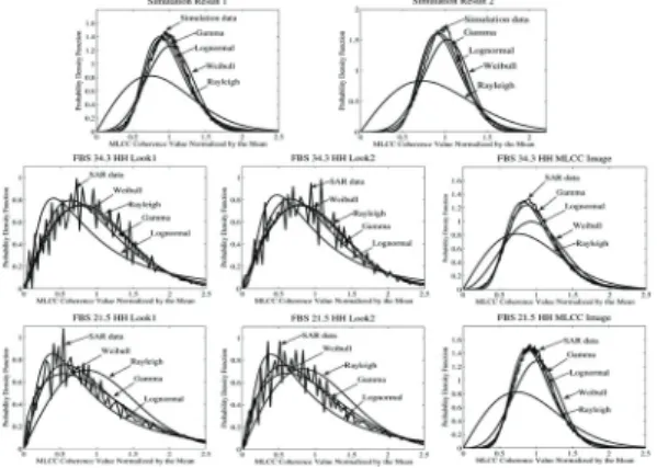
ABSTRACT ... In the small ship detection experiment in 2006 by PALSAR (Phased Array L-band Synthetic Aperture Radar) on board of ALOS (Advance Land Observing Satellite), we examined 4 ship detection algorithms including MLCC (Multi-Look Cross-Correlation) which is an useful technique to extract the images of ships embedded in heavy sea clutter. The result was that some boats were detected by thresholding MLCC coherence images under favourable conditions. However, it was also found that the threshold method was not suitable to automatically determine the threshold levels corresponding to desired FAR (False Alarm Rate) values. In order to overcome this problem and to improve the accuracy of ship detection by MLCC, we propose a new and simple technique of MLCC-CFAR (or Gamma-CFAR). In this method, CFAR (Constant False Alarm Rate) is applied to inter-look coherence images produced by MLCC. We tested this new algorithm using simulation and PALSAR data, and found substantial improvement in SNR (Signal to Noise Ratio) and FAR in comparison with the threshold method. In this letter, we summarize the MLCC-CFAR algorithm and the experimental results.

KEY WORDS: SAR, Ship detection, SNR, FAR, MLCC-CFAR

1. INTRODUCTION

After the launch of the SEASAT carrying L-band SAR in 1978, a substantial number of ship detection, classification and identification systems by spaceborne and airborne SARs have been reported [1], [2], [3]. Since SAR is a very effective means for monitoring of maritime traffic, fishing activity, ships responsible for ocean oil pollution, and illegally operating ships, in particular, for increasing marine crimes including smuggling and sea jacking by piracy. Among several current ship detection algorithms, MLCC is known to be able to extract the images of ships embedded in sea clutter [4].

During the calibration/validation stage of ALOS- PALSAR in 2006, we conducted an experiment of detecting small fishing boats whose sizes are comparable with the PALSAR resolution cells, with several algorithms including amplitude threshold, MLCC, CFAR (Constant False Alarm Rate) [5], and polarimetric analyses. It was pointed out, in the analysis based on MLCC, that when sub-aperture images contain correlated noise from sea surface, the detection probability decreases due to decreasing SNR (Signal to Noise Ratio) and increasing FAR [6]. Another disadvantage is that the method of thresholding MLCC coherence images was not adequate to automatically determine the threshold levels corresponding to desired FAR. To improve the accuracy of MLCC, we propose, in this paper, a novel method of ship detection by applying CFAR to MLCC coherence

images. The results indicate the increase of SNR up to about 12 dB and the reduction of FAR by 30% on average in comparison with those by the conventional method of thresholding the coherence images.

Section 2 presents the summary of the experiment in 2006 over the Tosa bay, Kochi, Japan. Section 3 is the main body of this paper, where the details of the proposed algorithm and the results of simulation and applications to PALSAR data are presented, followed by conclusions and suggestions for the future study in section 4.

2. SHIP DETECTION EXPERIMNT IN 2006 In the ship detection experiment in 2006, we deployed three types of small fishing boats simultaneously with PALSAR data acquisition in all ascending orbits. The hulls of all boats were made of FRP (Fiber Reinforced Plastics) with attached winches and fishing equipments on deck. The experiment was carried out as follows.

Before the time of PALSAR data acquisition, Type I

boat (Type Ia : 12.0 m, Type Ib : 14.6 m) was positioned

at 1 km away from the shoreline, followed by Type II

(Type IIa : 10.7 m, Type IIb : 11.9 m) and Type III (Type

IIIa : 8.0 m, Type IIIb : 9.2 m) boats separated by 50 m,

where the numbers inside the brackets correspond to the

boats' lengths. Type I boat started to cruise at 10 minutes

before the observation time with the cruising speed of 8

knots (4.12 m/s) in the direction away from the radar in

range direction. Then, Type II boat began to cruise followed by Type III boats with two minutes time interval with the same speed. We carried out the same experiment for 4 different PALSAR observation modes, namely FBS (Fine Beam Single) 21.5 HH, FBS 34.3 HH, FBD (Fine Beam Double) 41.5 HH/HV, and PLR (PoLaRimetric) 20.5 HH/HV/VH/VV. The numbers after the modes indicate the nominal off-nadir angles followed by the polarization modes. In the present work, we used the all 4 SAR data. The readers can view a photo of deployed small boats for instance, the parameters of 4 observation modes and meteorological data [6].

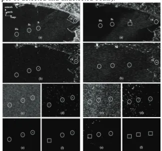
Figure 1 illustrates the results of ship detection from the FBS 34.3 HH (left side (a) to (f)) and FBS 21.5 HH (right side (a) to (f)) images respectively. In both figures, the images (a) and (b) correspond respectively to the amplitude images and the inter-look coherence magnitude images after applying MLCC to the sub- aperture images. In the figures, the image (c) indicates the enlarged coherence images of the area including boats, and the images (d) to (f) show the result after thresholding the coherence images (c) with the threshold parameter N = 2, 4, 6 respectively. The white circles indicate the detected boats; while the white square implies an undetected boat. The threshold value is calculated by

C

= C + N × σ

(1) where C is the mean value of coherence magnitude (or correlation coefficient), σ is the standard deviation, and

N is the parameter of threshold value. The coherence magnitude is computed from

1

2 1

2

1

−

= A A

A

C A (2)

where A and

A

are the look-1 and look-2 image amplitudes respectively for the case of two-look processing. In this study, the ensemble average was taken with a moving window of size 9 X 9 pixels.

The both images (d) to (f) in Figures 1 correspond respectively to the cases of N = 2, 4, 6. In the figures, white circles indicate detected boats and white squares imply undetected boats. The image size of each (a) is approximately 3.8 km in range direction (from left to right), and 2.1 km in azimuth direction (from bottom to top).

As shown in Table 1, the SNR value increases with increasing threshold parameter N from 0 to 6 because of reduced surrounding noise levels. This trend is visualized in the both (c)-(f) of Figure 1. However, for the FBS 34.3, the image of type IIIb was also thresholded out as in image (f) when N=6. Similarly, for the FBS 21.5 data, the image of Type IIIa disappeared as in image (e) when N = 4, and the images of all boats were thresholded out when N = 6. Then, the signal amplitude becomes zero with some remaining background noise, and hence SNR also becomes zero. This is the reason for the sudden drops in SNR in Table 1.

Table 2 shows decreasing FAR values as N increases by the threshold method. The numbers inside the brackets are the number of detected boats (see also Table 1 for the types of detected and undetected boats).

Figure 1. The results of ship detection from FBS 34.3 HH and FBS 21.5 HH. Each image is explained in the text.

Table 1. Comparison of SNR [dB] by thresholding the coherence images with different threshold parameters N and the proposed non-adaptive (MLCC-CFAR N) and adaptive (MLCC-CFAR A) methods.

Boat ype N=0 N=2 N=4 N=6 MLCC-CFAR N MLCC-CFRA A

FBS 34.3

Ib 25.6 32.0 59.9 64.7 62.5 66.9 IIa 22.9 29.6 59.5 6.34 61.3 65.7 IIIa 21.6 27.6 51.0 0.0 60.9 65.4 FBS 21.5

Ia 15.6 28.6 43.8 0.0 35.8 38.4 IIa 17.4 29.9 44.1 0.0 31.8 34.8 IIIa 15.6 22.8 0.0 0.0 30.6 31.6

In the same manner as for the SNR analysis, increasing N decreases the FAR values, but at the same time the number of detected boats decreases.

Thus, by applying a simple threshold technique to coherence images, SNR can be increased and FAR can be decreased, resulting in some improvement in detecting small ships. However, it is difficult to automatically determine the threshold parameter which is optimum to individual sub-scenes and there remains the main problem of noise arising from correlated scatters from sea surface. To overcome these problems, i.e., to determine threshold values for desired FAR and to improve the accuracy of MLCC (though background noise is still a problem), we propose a new method applying CFAR to the MLCC coherence images.

Table 2. Comparison of FAR by thresholding the

coherence images with different threshold parameters N

and the proposed non-adaptive (MLCC-CFAR N) and

adaptive (MLCC-CFAR A) methods. The numbers inside

the brackets show the number of detected boats

Data N=2 N=4 N=6 MLCC-CFAR N MLCC-CFRA A FBS 34.3 (3) 2.74E-2 (3) 7.31E-4 (2) 3.56E-4 (3) 4.56E-4 (3) 2.17E-4

FBS 21.5 (3) 3.06E-2 (2) 9.83E-4 (0) 2.50E-4 (3) 1.33E-2 (3) 8.88E-3

3. MLCC-CFAR TECHNIQUE 3.1 Methodology

Figure 2 shows the flowchart of the proposed method for ship detection, which we call MLCC-CFAR. The procedure up to the production of the coherence images from sub-aperture amplitude images is the same as for the previous MLCC method, i.e., 2-look sub-images are produced by using two non-overlapping sub-reference signals and the look-1 and look-2 amplitude images are cross-correlated using 9 X 9 moving window to yield the coherence image.

In order to apply CFAR to the MLCC coherence image, it is necessary to find a PDF (Probability of Density Function) which fits best to the coherence image. In this study, we consider 4 distribution models: Gamma, Weibull, Lognormal and Rayleigh distribution. The choice of a best-fitted PDF was made by comparing the AIC (Akaike Information Criterion) value [7]. The AIC values for the goodness-of-fit can be computed by two ways; one is to use the data over an entire sub-scene such as Figure 1 (c), and the other is to use the data within a moving window of size smaller than the sub-scene. The reason for the latter is that the statistical property may vary depending on the local image areas. The value of the AIC itself is not significant, but the differences in AIC values for different PDFs are important. A model which yields minimum AIC is regarded as the best fit. Once the best selection of PDF is made, the next step is to determine the parameters for estimated PDF by MLE (Maximum Likelihood Estimation) and calculating the threshold value by numerical integration. For computing the threshold, PFA (Probability False Alarm) was given as 1.0 E-4 for FBS 34.3 and 5.0 E-3 for FBS 21.5. Again, as for the selection of PDF by AIC, there are two ways of computing the threshold value, i.e., using the entire sub- scene and the data within a smaller moving window. We call the former as “non-adaptive” MLCC-CFAR and the latter as “adaptive” MLCC-CFAR.

Figure 2. Flowchart of the proposed MLCC-CFAR method for ship detection.

3.2 Simulation of MLCC-CFAR

Before applying MLCC-CFAR to PALSAR data, we first performed a simulation study, in which two statistically uncorrelated sub-aperture amplitude images of size 400 X 400 were produced. The Weibull distribution was assumed for the amplitude fluctuations

Figure 3. The results of PDF estimation including simulations and real sub-aperture PALSAR amplitude and MLCC coherence images. See text for detail.

because the PALSAR data used in this study were found to follow the Weibull distribution [5] as also shown in Figure 3. It is a versatile distribution function to describe sea clutter, having Rayleigh distribution as a limiting case [5]. The simulation results are shown in the top row in Figure 3 for PDFs of coherence images from two trials.

In Figure 3, the PDFs of coherence images were computed by correlating two simulated sub-aperture images obeying Weibull distribution with the shape parameters 1.9 and 2.1 for the 1st trial in the top-left, and 1.5 and 1.7 for the 2nd trial in the top-right. In both trials, the Gamma distribution was found to fit best to the coherence images. The quantitative comparison by AIC is similar to PDFs for both trials. The smallest AIC values were Gamma distribution computed from the whole coherence image 400 X 400 pixels. The largest percentage of being a best fit when the moving window of size 100 X 100 was Gamma distribution, too. Thus, from the simulation result, it is concluded that the coherence image computed from two Weibull-distributed amplitude images obeys Gamma distribution, and the technique may also be called the Gamma-CFAR.

3.3 Application to PALSAR data

The MLCC-CFAR or Gamma-CFAR algorithm is now applied to the four sets of PALSAR data. The PDFs of look-1 and look-2 image amplitude are shown in the left and middle graphs of the middle row in Figure 4 for FBS 34.3, and those graphs of the bottom row for FBS 21.5.

The smallest AIC values for look-1 and look-2 images of

FBS 21.5 and 34.3 are those of Weibull distribution with

the shape parameter of 1.52 and 1.72 respectively for

FBS 21.5, and 1.94 and 1.92 for FBS 34.3. Thus, the real

sub-aperture PALSAR images are predominantly Weibull-distributed.

The results of the distribution estimate of coherence images are shown in the right columns of middle and bottom graphs of Figure 4. The AIC values of the whole images are smallest for Gamma distribution, and the numbers of being a best fit using a moving window are largest (average 87 % for the all modes) among four distribution functions. It should, however, be noted that the results of taking local statistics showed that the log- normal distribution was a best fit with average 13 % for the all modes. In the present study, we assume Gamma distribution for the noise model for the inter-look coherence image of PALSAR data.

Having selected the noise model, we determined the parameters of the distribution function by MLE, and computed the threshold values from numerical integration. The non-adaptive and adaptive MLCC- CFAR algorithms were then applied to the inter-look coherence image. The results are shown in Figure 4, where (a) and (b) are the images after non-adaptive and adaptive MLCC-CFAR respectively for the FBS 34.3 data; and (c) and (d) are those after the corresponding MLCC-CFAR for the FBS 21.5 data. Comparison of SNR is shown in Table 1. Both the non-adaptive and adaptive MLCC-CFAR showed better performance than the simple thresholding method. The SNR values after non-adaptive MLCC-CFAR are lower than the value after thresholding with N = 6 for FBS 34.3 and N = 4 for FBS 21.5. However, one boat was undetected for both cases by thresholding.

For FBS 34.3, the mean SNR over all three detected boats improved to 56.8 dB for N = 4 from 23.4 dB for coherence image; and further improved to 61.6 dB and 66.0 dB after non-adaptive and adaptive MLCC-CFAR respectively. Similarly, for FBS 21.5, the mean SNR increased to 27.1 dB for N = 2 from 16.2 dB for coherence; and increased further to 32.7 dB and 34.9 dB after applying non-adaptive and adaptive MLCC-CFAR respectively. The SNR for FBS 21.5 is not as large as that for FBS 34.3 because of coarse ground-range resolution.

This difference can be seen in Figure 4, in which there still remain some scattered noise in the coherence images of (c) and (d) after MLCC-CFAR for FBS 21.5.

Table 2 shows the comparison of the FAR values. For FBS 34.3, the FAR values decreased to 4.56E-4 and 2.17E-4 respectively after non-adaptive and adaptive MLCC-CFAR from 2.74E-2 N = 2 and 7.31E-4 for N = 4.

For N =6, the FAR value decreased to 3.56E-4, but only two boats were detected. Similarly, further decrease in FAR after MLCC-CFAR can be seen for FBS 21.5, although the amount of decrease is not as large as for FBS 34.3 for the same reason as for the case of SNR.

4. CONCLUSION AND FUTURE WORK A technique of MLCC is known to be able to extract the images of ships embedded in clutter by thresholding coherence images produced by cross-correlating sub-

aperture SAR images. The basic idea is the strong inter- look correlation of deterministic targets such as ships, and weak correlation of surrounding noises. One of the problems of this method is that it is difficult to determine the correct threshold values. In the present paper, we proposed a new simple technique to determine the optimum threshold values corresponding to desired FAR and to improve MLCC, by applying CFAR to the MLCC

Figure 4. Images after MLCC-CFAR. Each image is explained in the text.

coherence images. We tested the proposed method of MLCC-CFAR using simulation and ALOS-PALSAR data containing small fishing boats of sizes comparable with the SAR resolution cells. The results showed that substantial improvement was made by MLCC-CFAR in both the SNR and FAR values in comparison with the threshold method, and that the adaptive MLCC-CFAR was superior to the non-adaptive MLCC-CFAR. In the present study, the Gamma distribution was found to model the noise statistics of the coherence images computed from the Weibull-distributed sub-aperture images of sea surface. This finding was based on the simulation and actual PALSAR data. It is a subject of future work to investigate the theoretical relation between the distribution functions in sub-aperture and coherence images.

REFERENCES

[1] W. H. Munk, P. Scully-Power, and F. Zachariasen, 1987. “Ships from space,” Proc. Roy. Soc. London. A, vol.412, pp.231-254.

[2] T. N. Arnesen and R. B. Olsen, 2004. Literature Review on Vessel Detection, FFI/RAPPORT-2004/02619, Forsvarets Forskningsinstitutt (Norwegian Defence Research Establishment), Kjeller, Norway,.

[3] H. Greidanus, DECLIMS : Requirements for Future Systems, Joint Research Center, European Commission DECLIMS homepage. \\http://declims.jrc.ec.europa.eu.

[4] K. Ouchi, S. Tamaki, H. Yaguchi, and M. Iehara, 2004. “Ship detection based on coherence images derived from cross-correlation of multilook SAR images, IEEE Trans. Geosci. Remote Sens. Lett., vol.1, pp.184-187,.

[5] M. Sekine and Y. Mao, 1990. Weibull Radar Clutter, Peter Peregrinus, London.

[6] S-I. Hwang, H. Wang, and K. Ouchi, 2009.

“Comparison and evaluation of ship detection and

identification algorithms using small boats and ALOS- PALSAR,” IEICE Trans. Commun., vol.E92-B, no.12, (Accepted for publication).

[7] H. Akaike., 1973. “Information theory and an extension of the maximum likelihood principle,” Proc.

2nd International Symposium on Information Theory,

pp.267-281,.