Comparative Usefulness of Naver and Google Search Information in Predictive Models for Youth Unemployment Rate in Korea

(1)

Comparative Usefulness of Naver and Google Search Information in Predictive Models for Youth Unemployment Rate in Korea

Jae Un Jung

Assistant Professor, Department of Management Information Systems, Dong-A University

한국 청년실업률 예측 모형에서 네이버와 구글 검색 정보의 유용성 분석

정재운

동아대학교 경영정보학과 조교수

Abstract Recently, web search query information has been applied in advanced predictive model research. Google dominates the global web search market in the Korean market; however, Naver possesses a dominant market share.

Based on this characteristic, this study intends to compare the utility of the Korean web search query information of Google and Naver using predictive models. Therefore, this study develops three time-series predictive models to estimate the youth unemployment rate in Korea using the ARIMA model. Model 1 only used the youth unemployment rate in Korea, whereas Models 2 and 3 added the Korean web search query information of Naver and Google, respectively, to Model 1. Compared to the predictability of the models during the training period, Models 2 and 3 showed better fit compared with Model 1. Models 2 and 3 correlated different query information. During predictive periods 1 (continuous with the training period) and 2 (discontinuous with the training period), Model 3 showed the best performance. During predictive period 2, only Model 3 exhibited a significant prediction result. This comparative study contributes to a general understanding of the usefulness of Korean web query information using the Naver and Google search engines.

Key Words : Korean Web Query, Predictor, Youth Unemployment, Time Series Prediction, Machine Learning

요 약 최근 고급 예측모형 연구에 웹 검색 정보가 활용되고 있다. 세계 웹 검색시장에서 구글이 절대적 우위를 점하고 있지만, 국내 웹 검색시장에서는 네이버가 절대적 우위를 보이고 있다. 이러한 특성을 토대로 본 연구는 예측모형을 활용하 여 구글과 네이버의 한국어 검색 정보에 대한 유용성을 비교해 보고자 한다. 이를 위해 ARIMA 모형을 활용하여 세 가지의 한국 청년실업률 예측 시계열 모형을 개발하였다. 모형1은 한국 청년실업률 데이터만 사용하였으며, 모형2와 3은 모형1에 네이버와 구글의 검색어 정보를 각각 추가하였다. 모형 훈련기간에서는 모형1보다 모형2와 3이 더 우수한 예측력을 보였다.

모형2와 3은 서로 다른 검색어 정보와 상관관계를 보였으며, 예측기간 1과 2에서 모형3이 가장 좋은 성능을 보였다. 예측기 간 2에서는 모형 3만 유의미한 예측결과를 나타내었다. 이 비교 연구는 네이버와 구글 검색엔진을 이용한 한국어 웹 검색 정보의 유용성을 이해하는 데 도움을 준다.

주제어 : 한국어 웹 검색어, 예측변수, 청년실업률, 시계열예측, 머신러닝

*This work was supported by the Ministry of Education of the Republic of Korea and the National Research Foundation of Korea (NRF-2017S1A5A8018867)

*Corresponding Author : Jae Un Jung([email protected]) Received June 15, 2018

Accepted August 20, 2018

Revised July 2, 2018 Published August 28, 2018

(2)

1. Introduction

Web search logs can be used to understand diverse individual considerations and social phenomena [1,2].

Initially, web search information was used to identify past phenomena; however, such information has recently been used to identify real-time or predictable issues [3-5]. If web search query information trends demonstrate similarity with social trends, it is assumed that information can be used as an effective predictor.

Based on this assumption, web search query information has been applied to predictive modeling for a wide range of topics, e.g., influenza and unemployment rates [6,7].

Most web search query information used in predictive modeling is relative frequency scaled from 0 to 100 in a form provided by web search engines such as Google [8]. Retrieving actual frequency data directly from web search engine databases can be problematic due to security and system stability issues, which limits the practical application of such data [9]. Relative frequency data represent trends in web search logs and freely available; however, the relative value is less accurate than the actual frequency value [10].

Google commands 90% of the global web search market, whereas the Baidu (Chinese) and Naver (Korean) search engines command approximately 1%

[11]. However, Baidu and Naver dominate the Chinese and Korean markets, showing 70% and 80% market shares in those regions, respectively [12,13]. Local and linguistically distinct search engines, such as Baidu and Naver, are preferable for predictive modeling of local issues [14,15].

Based on this characteristic, this study compared the usefulness of Korean query information from Naver and Google to predict Korea’s youth unemployment rate using three predictive models. The autoregressive integrated moving average (ARIMA) model technique, widely used for time series analysis [16], was employed to construct a baseline predictive model (Model 1) using Korean youth unemployment data from Statistics

Korea [17], and the baseline model was extended using Korean web search query information from Naver (Model 2) and Google (Model 3). By performing comparative analysis, this study was able to identify that Models 2 and 3 exhibited correlations with different query information. Further, Model 3 outperformed Model 2 during predictive periods 1 and 2.

2. Model1: Baseline Predictive Model for Korea’s Youth Unemployment Rate

In this study, the baseline predictive model referenced the ARIMA predictive model for Korea’s youth unemployment proposed by Kwon and Jung [18].

However, in their model, the youth unemployment data ([18]; Table 1) were updated by Statistics Korea.

Therefore, raw time-series youth unemployment data from May 2010 to April 2015 (60 months) were obtained from Statistics Korea (See Table 1). The data are plotted in Fig. 1(a). The first 54 months of data were used as the training dataset, and data from the last six months were used as the test dataset.

The logarithmized (normalized) result of the collected raw data is shown in Fig. 1(b).

2010 2011 2012 2013 2014 2015

January 8.5 8.0 7.5 8.7 9.1

Feburary 8.5 8.3 9.0 10.8 11.0

March 9.4 8.3 8.5 9.9 10.7

April 8.7 8.4 8.3 10.0 10.2

May 6.4 7.3 8.0 7.4 8.7

June 8.2 7.6 7.7 7.9 9.5

July 8.4 7.6 7.3 8.2 8.9

August 7.0 6.3 6.4 7.6 8.4

September 7.2 6.3 6.7 7.7 8.5

October 7.0 6.7 6.8 7.8 8.0

November 6.4 6.7 6.7 7.5 7.9

December 8.0 7.7 7.5 8.5 9.0

Table 1. Korea’s youth unemployment rate (%)

(3)

Fig. 1. Youth unemployment rate in Korea (%)

Fig. 2. ACF and PACF after normalization

Fig. 3. ACF and PACF after differencing

Fig. 4. ACF and PACF after seasonal differencing

(4)

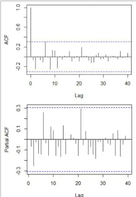
Using the normalized data, autocorrelation functions (ACF) and partial autocorrelation functions (PACF) were calculated step by step. Fig. 2 shows the obtained ACF and PACF values. Fig. 3 shows the result obtained after first non-seasonal differencing (removing trend), and Fig. 4 shows the result obtained after seasonal differencing (removing seasonality, period = 12).

The residual ACF and PACF values are within the confidence intervals (blue dotted lines). Referred to as white noise, this status indicates that no further processing is required to obtain stationary and non-autocorrelated youth unemployment data [19].

Based on the ACFs and PACFs that have been plotted of Figs. (2)–(4) and diagnostic plotting with the sarima function in R [20], the following models can be estimated to be alternative models (See Table 2).

In Table 2, ARIMA(1,0,0)(1,0,0)12 exhibited the lowest Akaike information criterion (AIC) [21];

therefore, this study selected Model 1 as the final estimated model. Fig. 5 depicts the diagnostic result of Model 1.

Table 3 shows the coefficients of the estimated ARIMA model, i.e., Model 1, which includes a non-seasonal autoregressive (AR)(1) term and a seasonal AR(1) term with the seasonal period, s = 12.

Model AIC

1 ARIMA(0,1,0)(1,0,0)12 -118.02

2 ARIMA(0,1,0)(0,0,1)12 -110.05

3 ARIMA(1,0,0)(1,0,0)12 -127.35

4 ARIMA(1,0,0)(0,1,0)12 -73.19

5 ARIMA(1,0,0)(0,0,1)12 -121.42

Table 2. Alternative models

Coefficients SE t Value p Value

AR1 0.7379 0.0904 8.1583 0

SAR1 0.7565 0.0900 8.4070 0

Table 3. Estimated coefficients of Model1

The non-seasonal AR(1) and seasonal AR(1) are represented by Equations (1) and (2), respectively, and Model 1 is represented by Equation (3) [22].

Fig. 5. Diagnostic plots of Model 1

(5)

   _ (1)

^   _^ (2)

 _^ __   _ (3)

Here, for simplicity, let_ _ . Then, Equation (4) can be obtained by multiplying the two AR components and pushing all but _ to the right side [22].

_ __{  } __{  }  ___{  } _ (4)

Here, Model 1 is simply represented by the following regression equation.

   ln_  _ _ln_{  } 

_ln_{  }  _ln _{  }  _

(5)

Table 4 shows the estimated coefficients of Model 1.

The estimated Model 1 (represented by Equation (6)) shows explanatory power of 78.2% (R²: 0.782).

Predictor Unstandardized β

(Std. Error) Standardized β t Sig.

Constant .114(.204) .558 .581

ln(Xt-1) .799(.100) .803 7.957 .000

ln(Xt-12) .627(.112) .515 5.619 .000

ln(Xt-13) -.479(.127) -.407 -3.764 .001

R²(Adjusted) .798(.782)

Std. Error of the Estimate .0583361208 Significance of the Regression

Model .000

Table 4. Estimated coefficients of Model1

   ln_   ln_{  } 

ln_{  }  ln_{  }  _ (6)

3. Model2: Estimating Predictive Models Using Naver Query Information

To improve Model 1, this study estimated the predictive models using Korean Naver query information (Model 2). To use web search query information as a predictor, this study selected 18 Korean keywords (Q1-Q18) associated with Korea’s

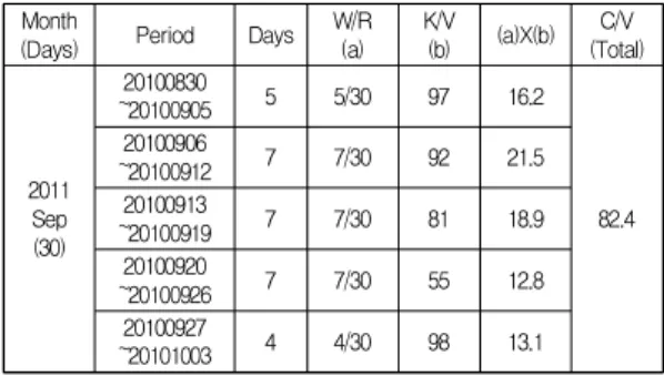
youth unemployment rate (see Table 5), used in Kwon and Jung [18], and retrieved the 18 weekly Naver search query information (relative frequency scaled from 0 to 100) during the same period defined in Table 1.

Among the 18 Naver search query information, time unit transformation (weekly to monthly) of the Naver query information was performed (Table 6 shows an example) to identify correlated query information.

Then, a correlation analysis was performed. Thus, five queries (Q1, Q3, Q11, Q17, and Q18) showed correlation

>0.5 (See Table 7). The selected Naver search queries were the same as those reported by Kwon and Jung [18]; however, the correlation values were slightly different.

Keywords Keywords

Q1 기업(company) Q10 정규직

(permanent position)

Q2 경제(economy) Q11 임대주택(rental house)

Q3 고용(employment) Q12 지원(support)

Q4 대학원진학(enter-

graduate-school) Q13 실업(unemployment)

Q5 정부(government) Q14 청년창업(youth startup)

Q6 취업(get-a-job) Q15 청년실업(youth

unemployment)

Q7 대학원(graduate school) Q16 청년실업률(youth

unemployment rate)

Q8 일자리(job) Q17 청년취업(youth

employment)

Q9 입대(join-the-army) Q18 실업급여

(unemployment benefits) Table 5. 18 keywords associated with Korea’s youth

unemployment rate ([18]; Fig.6)

Month

(Days) Period Days W/R

(a) K/V

(b) (a)X(b) C/V (Total)

2011 Sep (30)

20100830

~20100905 5 5/30 97 16.2

82.4 20100906

~20100912 7 7/30 92 21.5

20100913

~20100919 7 7/30 81 18.9

20100920

~20100926 7 7/30 55 12.8

20100927

~20101003 4 4/30 98 13.1

※ W/R: weighted rate, K/W: keyword value, C/V: converted value

Table 6. Time unit conversion of web search query information ([18]; Table 4)

(6)

Query Correlation

Q1 .637^**

Q3 .743^**

Q11 .630^**

Q17 .752^**

Q18 .831^**

**Correlation is significant at the 0.01 level (2-tailed)

Table 7. Correlated Naver search queries (>0.5)

Considering the five Naver query information as an additional predictor (ln(Qtk

)), Model 2 is expressed as follows.

ln_  __ln_{  }  _ln_{  } 

_ln_{  } _{  }



^ ^^^ln^^^^{  }^^

(7)

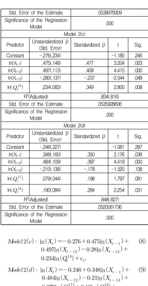
Models 2(a) and 2(b) in Table 8 were determined using the stepwise method in SPSS Statistics 25. Here, ln(Xt-12) and ln(Xt-13) were not included in both models.

Models 2(c) and 2(d) were determined via the enter method using the Naver query information selected in Model 2(a) (Q18) and 2(b) (Q17 and Q18), respectively.

Models 2(c) and 2(d) showed better explanations compared with Model 1 without query information (Model 2(c): 83.4%, Model 2(d): 84.8%).

  ln_   ln_{  } 

ln_{  }  ln _{  } 

ln_^ _

(8)

  ln_   ln_{  } 

ln_{  }  ln_{  } 

ln_^ ln_^  _ (9)

The estimated Models 2(c) and 2(d) (Equations (8) and (9), respectively) are compared to Model 3 in terms of predictability using Google search query information in Section 5.

4. Model3: Estimating Predictive Models Using Google Query Information

This study has discussed the estimation of predictive models using Korean Google query information (Model 3). In the same manner used for Model 2, this study retrieved weekly Google search query information during the same period as the

Model 2(a) Predictor Unstandardized β

Constant -.551(.223) -2.472 .018

ln(Xt-12) .429(.104) .352 4.122 .000

ln(_^) .444(.057) .662 7.742 .000

R²(Adjusted) .787(.775)

Model .000

Model 2(b) Predictor Unstandardized β

Constant -.398(.209) -1.901 .065

ln(Xt-12) .432(.095) .355 4.559 .000

ln() .121(.041) .304 2.969 .005

ln() .291(.073) .434 3.977 .000

R²(Adjusted) .828(.814)

Table 8. Estimated coefficients of Model 2

Model .000

Model 2(c) Predictor Unstandardized β

Constant -.276(.234) -1.180 .246

ln(Xt-1) .475(.148) .477 3.204 .003

ln(Xt-12) .497(.113) .408 4.415 .000

ln(Xt-13) -.280(.137) -.237 -2.044 .048

ln(_^) .234(.083) .349 2.800 .008

R²(Adjusted) .834(.816)

Model .000

Model 2(d) Predictor Unstandardized β

Constant -.246(.227) -1.081 .287

ln(Xt-1) .348(.160) .350 2.176 .036

ln(Xt-12) .484(.109) .397 4.419 .000

ln(Xt-13) -.210(.138) -.178 -1.520 .138

ln(_^) .079(.044) .198 1.797 .081

ln() .190(.084) .284 2.254 .031

R²(Adjusted) .848(.827)

Model .000

(7)

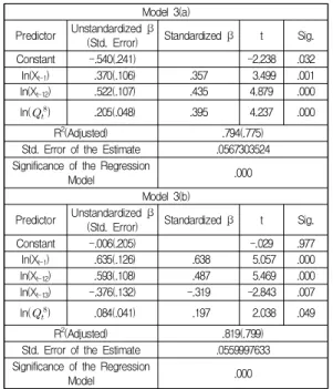
Korean youth unemployment data in Table 1 using the 18 keywords given in Table 5. Further, this study transformed the time unit of the Google search query information from weekly to monthly. Correlation analysis was then performed. Thus, Q6, Q8, and Q17 correlated (>0.5) the youth unemployment rate in Korea (See Table 9).

Models 3(a) and 3(b) were then estimated using the selected Google query information (Q6, Q8, and Q17).

Model 3(a), in Table 10, was estimated using the stepwise method in SPSS Statistics 25.

Query Correlation

Q6 .549^**

Q8 .664^**

Q17 .530^**

**Correlation is significant at the 0.01 level (2-tailed)

Table 9. Correlated Google search queries (>0.5)

Model 3(a) Predictor Unstandardized β

Constant -.540(.241) -2.238 .032

ln(Xt-1) .370(.106) .357 3.499 .001

ln(Xt-12) .522(.107) .435 4.879 .000

ln() .205(.048) .395 4.237 .000

R²(Adjusted) .794(.775)

Model .000

Model 3(b) Predictor Unstandardized β

Constant -.006(.205) -.029 .977

ln(Xt-1) .635(.126) .638 5.057 .000

ln(Xt-12) .593(.108) .487 5.469 .000

ln(Xt-13) -.376(.132) -.319 -2.843 .007

ln() .084(.041) .197 2.038 .049

R²(Adjusted) .819(.799)

Model .000

Table 10. Estimated coefficients of Model 3

Here, only Q8 was included; however, ln(Xt-13) was excluded. Model 3(b) was determined via the enter method using the Google query information, Q8, selected in Model 3(a).

Model 3(b) showed better explanation (R²: 81.9%) than Model 1 (78.2%) without query information but poorer explanation than Models 2(c) and 2(d) using the Naver query information (83.4% and 84.8%, respectively). Model 3(b) is expressed as follows.

  ln_   ln_{  } 

ln_{  }  ln_{  } 

ln_^ _

(10)

5. Predictive and Comparative Analysis

During the training period, this study identified that Models 2 and 3 using the Naver and Google query information showed better fit than Model 1, which only used the youth unemployment rate data. Compared to Models 2 and 3, Model 2(d) showed the best fit to the real data.

This section discusses a two-phase predictive comparison of Model 1, Model 2(c), Model 2(d), and Model 3(b). Here, predictive period 1 is from November 2014 to April 2015; this period is continuous (neighboring) with the training period (May 2010 to October 2014). Predictive period 2 is from January 2016 to December 2017 (24 months), and this period is not continuous (discrete) with the training period.

5.1 Predictability during Predictive Period 1 To compare the usefulness of the Naver and Google query information during predictive period 1, the coefficient of determination (R²) and root mean squared prediction error (RMSE) of Model 1, Model 2(c), Model 2(d), and Model 3(b) were calculated. Note that the coefficient of determination only shows the magnitude of the association; thus, for a more accurate comparison, the RMSE was also analyzed [23,24].

The coefficient of determination is given in Equation (11), where y is the real unemployment rate,  is the mean of y, and  represents the predicted values [25].

(8)

^_{   }

  ^

  ^

 (11)

With the RMSE, a lower value means better predictive performance [26]. Here, the prediction error is determined by the difference between the predicted and real values using Equation (12) [27].

_{ }



_{  }



^ ^^^{ }^^^^^ ^^^^^^ ⁽¹²⁾

During predictive period 1, Model 3(b) using the Google query information demonstrated the highest coefficient of predictive determination value (R²: 0.881).

Differing from the result obtained in the training period, Model 1 (0.872) without web query information showed the second highest value, followed by Models 2(c) (0.845) and 2(d) (0.834), which used the Naver query information. The results are shown in Table 11. In terms of RMSE, Model 3(b) showed the best performance (lowest value: 0.0396), followed by Models 1 (0.0410), 2(c) (0.0452), and 2(d) (0.0468).

R² MSE RMSE

Model 1 .872 .0017 .0410

Model 2(c) .845 .0020 .0452

Model 2(d) .834 .0022 .0468

Model 3(b) .881 .0016 .0396

Table 11. Models predictability during predictive period 1

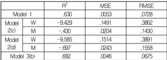
5.2 Predictability during Predictive Period 2 Unlike predictive period 1, predictive period 2 (24 months; from January 2016 to December 2017) is discontinuous with the training period.

To simulate the predictive models during this period, this study retrieved the youth unemployment rate in Korea from Statistics Korea (see Table 12), as well as the Naver (Q17 and Q18) and Google (Q8) weekly query information during the period corresponding to predictive period 2. The weekly web search query

information was transformed to match the monthly youth unemployment data in the manner shown in Table 6. During predictive period 2, all models demonstrated worse explanations than those of predictive period 1.

The coefficient of determination values for Models 3(b) and 1 were 0.682 and 0.630, respectively (Table 13), and those of Models 2(c) and 2(d) were negative (-9.429 and –9.585, respectively). The negative values indicated that the regressive model using the mean value of the real data was better than Models 2(c) and 2(d) (  ^<  ^ in Equation (11)) [28].

Thus, this study analyzed the RMSE of Models 2(c) and 2(d) by collecting another Naver monthly query information that did not require transformation of the data type to monthly. As a result, the coefficients of determination were improved; however, the values were still negative (-0.430 and –0.697).

Consequently, for predictive period 2, Models 2(c) and 2(d) using the Naver search query information rejected.

2016 2017

January 9.5 8.6

Feburary 12.5 12.3

March 11.8 11.3

April 10.9 11.2

May 9.7 9.2

June 10.3 10.4

July 9.3 9.3

August 9.3 9.4

September 9.4 9.2

October 8.5 8.6

November 8.1 9.2

December 8.4 9.2

Table 12. Korea’s youth unemployment rate during predictive period 2 (%)

R² MSE RMSE

Model 1 .630 .0053 .0728

Model 2(c)

W -9.429 .1491 .3862

M -.430 .0204 .1430

Model 2(d)

W -9.585 .1514 .3891

M -.697 .0243 .1558

Model 3(b) .682 .0046 .0675

Table 13. Model predictability during predictive period 2

(9)

In terms of RMSE, Model 3 showed the lowest error (0.0675), followed by Model 1 with 0.0728 (See Table 13).

Through these predicted results, this study identified that Model 3(b) using Google web search query information outperformed Models 2(c) and 2(d) during predictive periods 1 and 2.

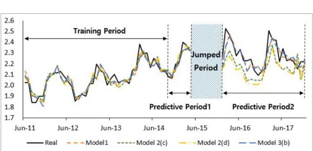
Fig. 6 plots the graphs of the predictive models over the training period, predictive period 1, and predictive period 2. As shown in Fig. 6, during predictive period 2, the results of Models 2(c) and 2(d) were simulated using the Naver monthly query information as reference.

6. Discussion

Even though the Google search engine dominates the worldwide web search market, in the Korean market, the Naver search engine has a dominant share.

Based on the characteristics of both search engines, this study compared the usefulness of Korean web search query information from both Naver and Google relative to the prediction of the youth unemployment rate in Korea.

As a result, web search query information from both Google and Naver improved the naive Model 1 using

only youth unemployment data. However, Model 3(b) with Google query information showed better predictability. In addition, Models 2(c) and 2(d) showed good performance during predictive period 1 (continuous with the training period) but demonstrated greater errors than the regressive model with the average value of Korea’s youth unemployment rate during predictive period 2, which is discontinuous with the models’ training period.

To generalize the findings of this study, a follow-up with more diverse topics is required; however, in the current study, Korean query information from Google showed better performance relative to improving a predictive model of the youth unemployment rate in Korea. In addition, our comparative analysis has identified that the performance of the predictive models differed depending on the duration of the web query information. Thus, for more accurate predictions, more stable and effective predictive techniques, such as refining and conjoining web search query information, will be the focus of future study.

REFERENCES

[1] B. J. Jansen. (2006). Search Log Analysis: What It Is, What’s Been Done, How to Do It. Library &

Fig. 6. Prediction performance for Korea’s youth unemployment rate by model (%)

(10)

Information Science Research, 28, 407-432. DOI : 10.1016/j.lisr.2006.06.005

[2] S. P. Jun, T. E. Sung & H. W. Park. (2016). Forecasting by Analogy Using the Web Search Traffic.

Technological Forecasting and Social Change, 115(1), 37-51. DOI : 10.1016/j.techfore.2016.09.014

[3] O. Y. Reiger. (2009). Search Engine Use Behavior of Students and Faculty: User Perceptions and Implications for Future Research. First Monday, 14(12). DOI : 10.5210/fm.v14i12.2716

[4] F. Wu, J. Madhavan & A. Halevy. (2011). Identifying Aspects for Web-Search Queries. Journal of Artificial Intelligence Research, 40(1), 677-700.

DOI : 10.1613/jair.3182

[5] B. J. Jansen, Z. Liu, C. Weaver, G. Campbell & M.

Gregg. (2011). Real Time Search on the Web: Queries, Topics, and Economic Value. Information Precessing and Management, 47(4), 491-506.

DOI : 10.1016/j.ipm.2011.01.007

[6] J. Ginsberg, M. H. Mohebbi, R. S. Patel, L. Brammer, M.

S. Smolinski & L. Brilliant. (2009). Detecting Influenza Epidemics Using Search Engine Query Data. Nature, 457, 1012-1014. DOI: 10.1038/nature07634

[7] N. Askitas & K. F. Zimmermann. (2009). Google Econometrics and Unemployment Forecasting. Applied Economics Querterly, 55(2), 107-120.

DOI : 10.3790/aeq.55.2.107 [8] Trends Help. Google(Online).

https://support.google.com/trends/answer/4365533?hl=en [9] Y. Zhang, B. J. Jansen & A. Spink. (2009). Time Series Analysis of a Web Search Engine Transaction Log.

Information Processing and Management, 45(1), 230-245. DOI : 10.1016/j.ipm.2008.07.003

[10] M. Schaefer, G. Sapi & S. Lorincz. (2018). The Effect of Big Data on Recommendation Quality. The Example of Internet Search. Berlin : Düsseldorf Institute for Competition Economics.

[11] Worldwide Desktop Market Share of Leading Search Engines from 2010 to April 2018. Statista(Online).

https://www.statista.com/statistics/216573/worldwide-m arket-share-of-search-engines/

[12] China Search Engine Market in Q1 2018; 79% Driven by Mobile Search. China Internet Watch(Online).

https://www.chinainternetwatch.com/24311/china-searc h-engine-market-q1-2018-79-driven-mobile-search/

[13] Debunking the Korean Search Engine Search Market Share in 2017. The Egg(Online).

http://www.theegg.com/seo/korea/korean-search-engine

-market-share-update-2017/

[14] K. Liu et. al. (2016). Using Baidu Search Index to Predict Dengue Outbreak in China. Scientific Reports, 6, Article No. 38040. DOI : 10.1038/srep38040

[15] C. M. Kwon, S. W. Hwang & J. U. Jung. (2015).

Application of Web Query Information for Forecasting Korean Unemployment Rate. Journal of the Korea Society for Simulation, 24(2), 31-39.

[16] G. Petris, S. Petrone & P. Campagnoli (2009). Dynamic Linear Models with R. NY : Springer.

[17] Statistics Korea(Online). http://www.index.go.kr [18] C. M. Kwon & J. U. Jung. (2016). Forecasting Youth

Unemployment in Korea with Web Search Queries.

LNCS 9870, 3-14.

DOI : https://doi.org/10.1007/978-3-319-46301-8_1 [19] G. E. P. Box, G. M. Jenkins, G. C. Reinsel & G. M.

Ljung. (2015). Time Series Analysis: Forecasting and Control. Hoboken : Wiley.

[20] SARIMA. RDocumentation(Online).

https://www.rdocumentation.org/packages/astsa/version s/1.8/topics/sarima

[21] Q. N. Tran & H. Arabnia (2015). Emerging Trends in Computational Biology, Bioinformatics, and Systems Biology: Algorithms and Software Tools. MA : Morgan Kaufmann.

[22] Time Series Analysis. PennState Eberly College of Science(Online).

https://newonlinecourses.science.psu.edu/stat510/node/67/

[23] J. Proppe & M. Reigher. (2017). Reliable Estimation of Prediction Uncertainty for Physicochemical Property Models. Journal of Chemical Theory and Computation, 13(7), 3297-3317. DOI : 10.1021/acs.jctc.7b00235 [24] S. Boslaugh. (2008). Encyclopedia of Epidemiology.

Thousand Oaks : SAGE Publications.

[25] D. L. J. Alexander, A. Tropsah & D. A. Winkler. (2015).

Beware of R²: Simple, Unambiguous Assessment of the Prediction Accuracy of QSAR and QSPR Models.

Journal of Chemical Information and Modeling, 55(7), 1316-1322. DOI : 10.1021/acs.jcim.5b00206

[26] R. Pelānek. (2017). Measuring Predictive Performance of User Models: The Details Matter. Adjunct Publication of the 25th Conference on User Modeling, Adaptation and Personalization (pp. 197-201). NY : ACM.

[27] T. Chai & R. R. Draxler. (2014). Root Mean Square Error (RMSE) or Mean Absolute Error (MAE)? – Arguments against Avoiding RMSE in the Literature. Geoscientific Model Development, 7(3), 1247-1250.

DOI : 10.5194/gmd-7-1247-2014

(11)

[28] What Is R Squared And Negative R Squared. Fairly Nearby(Online).

http://www.fairlynerdy.com/what-is-r-squared/

Jung, Jae Un(정재운) [정회원]

▪Feb. 2008 : Dong-A University, M,S. in MIS

▪Oct. 2010 : Dong-A University, Ph.D. in MIS

▪Mar. 2017 ～ Present : Dong-A University, Dept. of MIS, Assistant Professor

▪Research Area : System Dynamics, Advanced Analytics, Logistics Information Systems

▪E-Mail : [email protected]