Comparative Study on Surrogate Modeling Methods for Rapid Electromagnetic Forming Analysis

https://doi.org/10.5228/KSTP.2018.27.1.28

Comparative Study on Surrogate Modeling Methods for Rapid Electromagnetic Forming Analysis

Seungmin Lee ¹ , Beom-Soo Kang ¹ , Kyunghoon Lee ^#

(Received November 1, 2017 / Revised January 15, 2018 / Accepted January 19, 2018)

Abstract

Electromagnetic forming is a type of high-speed forming process to deform a workpiece through a Lorentz force. As the high strain rate in an electromagnetic-forming simulation causes infeasibility in determining constitutive parameters, we employed inverse parameter estimation in the previous study. However, the inverse parameter estimation process required us to spend considerable time, which leads to an increase in computational cost. To overcome the computational obstacle, in this research, we applied two types of surrogate modeling methods and compared them to each other to evaluate which model is best for the electromagnetic-forming simulation. We exploited an artificial neural network and we reduced-order modeling methods. During the construction of a reduced-order model, we extracted orthogonal bases with proper orthogonal decomposition and predicted basis coefficients by utilizing an artificial neural network. After the construction of the surrogate models, we verified the artificial neural network and reduced-order models through training and testing samples.

As a result, we determined the artificial neural network model is slightly more accurate than the reduced-order model.

However, the construction of the artificial neural network model requires a considerably larger amount of time than that of the reduced-order model. Thus, a reduced order modeling method is more efficient than an artificial neural network for estimating the electromagnetic forming and for the rapid approximation of structural simulations which needs repetitive runs.

Key Words : Electromagnetic Forming, Surrogate Modeling, Proper Orthogonal Decomposition, Artificial Neural Network

1. Introduction

Electromagnetic forming (EMF) is a high-speed forming technique that utilizes repulsive forces generated by opposite magnetic fields in contiguous conductors. Owing to high strain rates inducing transient effects, it is infeasible to estimate constitutive parameters for EMF. To identify constitutive parameters, we may employ inverse parameter estimation suggested in the prior studies[1, 2]. The parameter estimation process in Refs.[1, 2] was found time- consuming due to repetitive runs of EMF analysis implemented by LS-DYNA. To reduce the EMF simulation time, we adopted surrogate modeling to expedite constitutive parameter identification. The previous research

[1, 2] used reduced-order modeling (ROM) with proper orthogonal decomposition (POD) and kriging for the rapid approximation of EMF simulation; for details of kriging, please see Ref.[3]. In this research, we applied two different types of surrogate modeling methods to the EMF simulation in Ref.[2] for a comparison study. One is an artificial neural network (ANN) that imitates the information-processing structure of a human brain. In the literature, ANN modeling has been used for the design optimization of a composite structure [4~8] and a concrete structure[9]. The other is ROM with POD and ANN techniques. In the literature, POD was commonly used for the parameter identification of a finite element beam problem[10, 11] and damage mechanics systems[12~14].

1. Department of Aerospace Engineering, Pusan National University

# Corresponding author : Department of Aerospace Engineering, Pusan

National University, Email addresses: aeronova@pusan.ac.kr

For ROM, we extracted an orthonormal basis of EMF simulation outputs by POD and predicted basis coefficients by an ANN. In this paper, we denote a reduced-order model constructed with POD and an ANN as “POD-ANN” for convenience. To compare ANN and POD-ANN models, we evaluated the accuracy and efficiency of the two surrogate models.

Overall, the objective of this research is to examine the two surrogate models of EMF simulation in terms of accuracy and efficiency. The outline of this paper is as follows. Section 2 briefly describes EMF simulation along with the formulations of ANN and POD methods. Section 3 shows procedures to build surrogate models with training samples. Subsequently, Section 4 measures the accuracy of the surrogate models with training and testing samples.

Section 5 summarizes this paper and concludes which surrogate modeling is more effective.

2. Electromagnetic Forming Simulation and Formulations of Surrogate Modeling

2.1 Electromagnetic Forming simulation

For the surrogate modeling of EMF simulation, we used data obtained from the numerical simulation of the EMF free bulge test presented in Ref. [2]. The LS-DYNA simulation of the EMF free bulge test was conducted with an aluminum 1050-H14 specimen whose thickness is 1.0 mm. To set up the numerical simulation of the EMF free bulge test, we used the LS-DYNA electromagnetism module to carry out an electromagnetic-structural coupling simulation as depicted in Fig. 1. The simulation model and material properties of the EMF simulation are shown in Fig. 2 and Table 1, respectively. Detailed information regarding the simulation model is given in Ref. [2].

In abstract, the LS-DYNA EMF simulation can be represented as

 

y  f x; 

,

where y  R

, x  R

, and  

R are discretized coordinates of a deformed workpiece, discretized spatial coordinates, and flow stress, respectively. The flow stress



is a parameter of the EMF simulation and assumed to follow the modified Johnson-Cook model:

(a)

(b)

Fig. 1 (a) Coupled electromagnetic and structural analysis of an EMF free bulge test [2], (b) Experimental results of an EMF free bulge test [2]

Fig. 2 Finite element model of LS-DYNA EMF simulation [2]

Table 1 Material properties for LS-DYNA EMF simulation [2]

Properties Value Unit Coil

(copper) Resistivity 1.72e-8  m

Sheet (Al1050-H14)

Resistivity 2.82e-8  m Poisson’s ratio 0.35 -

Density 2980 kg/m

Elastic modulus 69.0 GPa





0

; , 1 ln

P n

f e

C P A B

C 

  



 

        

  (1)

where  , and  are strain and strain rate, respectively,

and A , B , n , C and P are parameters of 

_{. Since}

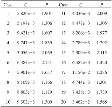
A , B , and n are parameters determined by a quasi- static tensile test, we can set C and P as surrogate model inputs. For the generation of training and testing samples, we utilized a specific domain of the material

parameters defined as follows:

 C P ,   D

  0.001,1.0    0.012, 2.2   R

[2]. Within the domain, each set of 20 samples was generated for both training and testing data in this study.

2.2 Artificial Neural Network

An artificial neural network is computational architecture that has been motivated by the biological neural network of a human brain. Similar to a human brain processing information with a vast number of neurons, an ANN interconnects artificial neurons to address various problems via artificial intelligence. To tackle a problem with an ANN, we need a backpropagation algorithm to train a neural network system. After training a neural network, we can apply the network to unexperienced situations. An ANN is commonly used in diverse applications involving data processing, such as function approximation and data classification [15]. In relation to forming simulation, ANN modeling is applicable to any materials, part shapes, and forming techniques as long as deformation is continuous with respect to input parameter changes; however, it tends to struggle with the increase of the output size. A detailed formulation on ANN is presented in Ref. [15].

2.3 Reduced-Order Modeling

Reduced-order modeling is a statistical technique to decrease the output dimension of mathematical models. In ROM, output prediction is accelerated by the reduction of basis vectors spanning the output space of the original model. Compared to the original model, a reduced-order model is typically slightly less accurate but greatly more efficient. Like ANN modeling, reduced-order modeling can be applied to any materials, parts shapes, and forming techniques if deformation is continuous with respect to input parameters.

Let y x   ;θ  R

be a large dimensional output associated with a spatial input x  R

and a parameter of interest θ  R

. In our application, y  R

represents

the discrete coordinates of a deformed workpiece, x  R indicates discretized spatial coordinates, and θ R 

denotes the two C and P parameters of the modified Johnson-Cook constitutive model. Suppose that we have a set of large dimensional outputs  ^{y x} 

^{ }

 

_populated

by variation in θ limited to a domain D such that θ   D R

. If a basis 

  

r

u x

is available, ^{y x}  ^{;θ  }



can be expressed as a linear combination of the basis as follows:

      ^{   }

1

;θ θ ,

r

i i

j j

j

y x a u x y



  

where

  ^θ  

^R

a

 is a basis coefficient corresponding to a basis vector u

  x  R

, and y is the sample mean of the output collection evaluated by

   

1

1

;θ

R

n

y y x

 

 . In general, we may drop the r  q insignificant basis vectors and employ the first q leading basis vectors to effectively represent ^{y x}  ^{;θ  }

 as

      ^{   }

1

;θ θ .

q

i i

j j

j

y x a u x y



   (2)

In this research, we achieved   u

as an orthonormal basis evaluated by POD and estimated   a

through an ANN. For details of POD, please see Refs. [16, 17].

3. Generation of surrogate models

3.1 Procedures of surrogate modeling

In this paper, we conducted the following steps for the construction of an ANN surrogate model. The first step is to generate training and testing data based on Latin hypercube and uniform random design, respectively. The second step is to build an ANN surrogate model to predict EMF simulation outputs. The next step is to verify the ANN surrogate model for training data. If the accuracy of the constructed ANN model is acceptable for training data, we verify the ANN model for testing data.

In the case of ROM, the first step is the same as that of

the ANN modeling process. The second step is to extract an

orthonormal basis by POD and to evaluate basis

coefficients by orthogonal projection. The next step is to

select a few dominant basis vectors based on eigenvalues

and to build a surrogate model of basis coefficients by

ANN modeling. The final step is to verify the basis

coefficient model for training and testing data. If the verification results are satisfactory, we construct a reduced- order model and then apply the same verification process to the reduced-order model.

3.2 Artificial neural network model

Fig. 3 Neural network architecture to approximate EMF simulation

With the help of the neural network toolbox in MATLAB, we constructed an ANN model with two hidden layers composed of 10 nodes as delineated in Fig. 3. The mathematical model behind a neural network is

 

0 0 0

,

e d c

l i kl jk ij i

k j i

y x h u g v f w x

  

     

                (3)

where x

and y

represent the parameters  C P ,   R

and the coordinates of deformed workpiece y  R

, respectively. To determine the neural networks system expressed in Eq. (3), we need to find weights and basis terms, v ^jk _and w _ij , in the layers. For this matter, we used Bayesian regularization backpropagation to train a neural network. For the 20 training samples, the ANN model construction took about 4 hours on a Mac 10.12 machine with 2.5 GHz Intel Core i7 and 16GB memory.

3.3 Reduced-order model 3.3.1 Basis extraction

To form a reduced-order model, we extracted the basis of the EMF simulation output with POD and calculated basis coefficients by orthogonal projection. To examine the significance of basis vectors, we normalized eigenvalues by their sum and sorted out the normalized eigenvalues in a decreasing order. As shown in Fig. 4, the sum of the first two leading eigenvalues is 0.9998, which means the first two basis vectors delineate 99.98% variations in the EMF simulation outputs. Therefore, we selected the two basis vectors to build a POD-ANN model. In Fig. 5(a), the first basis vector is associated with the central region of the EMF simulation output. On the other hand, the second

basis vector is related to the area near the flanges as shown in Fig. 5(b).

Fig. 4 Cumulative sums of normalized eigenvalues

(a)

(b)

Fig. 5 (a) The 1st dominant basis of EMF simulation outputs obtained with training samples, (b) The 2nd dominant basis of EMF simulation outputs obtained with training samples

3.3.2 Basis coefficients prediction

Fig. 6 Neural network architecture to approximate the

two basis coefficients of the reduced-order model

(a)

(b)

Fig. 7 (a) The 1st basis coefficient, (b) The 2nd basis coefficient

Fig. 8 EMF simulation outputs for the changes of C and P parameters

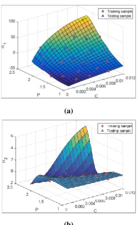
We estimated two basis coefficients by ANN modeling.

First, we built a neural network that involves two hidden layers as described in Fig. 6. To determine the weight and bias terms in Eq. (3), we conducted a backpropagation process as we did in Section 3.2. As a result, we obtained the basis-coefficient-predicting ANN model as shown in Fig. 7. Note that the first basis coefficient depicted in Fig.

7(a) tends to increase as the surrogate model inputs C

and P grow. Since the first basis vector in Fig. 5(a) is the reversed shape of a deformed workpiece, large C and P values lessen overall deformation. On the contrary, small C and P values result in the opposite effect. As an illustration, the effect of C and P on shape deformation is delineated in Fig. 8. The large and small C and P values produce small and large deformation, respectively. The POD-ANN model construction took just about a few seconds on the same computing environment described in Section 3.2.

4. Verification of surrogate models

4.1 Verification of surrogate models with training samples

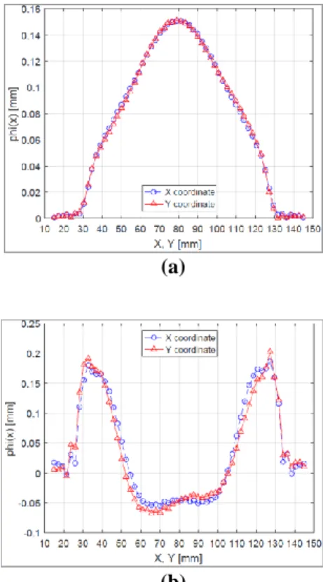
We examined the prediction accuracy of the constructed ANN and POD-ANN models for the training samples. As shown in Fig. 9, the predictions of both ANN and POD- ANN models are almost identical to that of the LS-DYNA EMF simulation for the training data. Note that the central region of the deformed shape in Fig. 9 is similar to the first basis vector in Fig. 6(a) in reverse. Along with the first basis vector, the POD-ANN model uses the second basis vector to compensate fluctuations near the edges to predict the overall deformation.

For numerical evaluation, we calculated the coefficient of determination ( R ), mean absolute relative error

(MARE), and maximum absolute relative error (max.ARE) defined as follows:

 

 

2

2 1

2 1

1

1 ˆ ,

ˆ ˆ

MARE= 1 , Max.ARE max ,

n

i i

i n i i

n

i i i i

i i i

y y

R

y y

y y y y

n y y







  



 



 



(4)

where y

, y ˆ

, y , and n denote the actual and predicted

responses, the sample mean of actual data, and the number

of samples, respectively. In Fig. 10, we summarized the

numerical verification results. In Fig. 10(a), the R values

of the two surrogate models are at least over 0.9982 and

almost one. Furthermore, MAREs are less than 0.25 and

spike to about 0.35 in Fig. 10(b); similarly, maximum

AREs mostly do not exceed 20 and rise up to about 30 in

Fig. 10(c).

(a)

(b)

Fig. 9 (a) EMF simulation outputs across the X direction (the 5th training case), (b) EMF simulation outputs across the Y direction (the 5th training case)

Next, we checked the worst prediction cases in terms of maximum AREs. We found that the 5th and 13th training cases were worst in case of the ANN and POD-ANN models, respectively. In particular, Fig. 10(b) shows that the 13th training case of the POD-ANN model resulted a significantly large maximum ARE value. According to Eq.

(4), a small exact value could cause a large maximum ARE.

The maximum ARE of the 13th training case turned out significantly large because of a small exact value, -2.4161e- 04, in the flange area; other than that, the 13th case exhibited prediction accuracy comparable with other training cases.

4.2 Verification of surrogate models with testing samples

We repeated the same verification process in Section 4.1 for testing samples. Note that both ANN and POD-ANN models do not show large errors as shown in Fig. 11.

(a)

(b)

(c)

Fig.10 (a) R of the surrogate models for the training

data (b) MARE of the surrogate models for the training data, (c) Maximum ARE of the surrogate models for the training data

In addition, we calculated R , MARE, and maximum

ARE values for testing samples and plotted the results in

Fig. 12. Figure 12(a) shows that R values of all testing

cases are close to one; R values are at least over 0.9982.

In Fig. 12(b), MAREs are mostly less than 0.4 and increase

up to about 1.7 for the 3rd testing case in the case of POD-

ANN. Similarly, in Fig. 12(c), maximum AREs are mostly

less than 40 except the 3rd testing case of POD-ANN,

which has a maximum ARE exceeding 160. For the worst

(a)

(b)

Fig.11 (a) EMF simulation outputs across the X direction (the 3rd testing case), (b) EMF simulation output across the Y direction (the 3rd testing case)

prediction case, we chose the 3rd testing case based on Fig.

12(b). Similar to Section 4.1, we noticed that a very small exact value of the 3rd testing case in the flange, 7.9850e-05, caused a large maximum ARE.

For further investigation, we checked the MARE and maximum ARE values in Figs. 10(b) and 10(c) for the training data and Figs. 12(b) and 12(c) for the testing data.

We found that the MARE and maximum ARE values of the ANN model are mostly a little smaller than those of the POD-ANN model. As for model construction cost, ANN modeling took tremendous amount of time compared to POD-ANN modeling; the former spent about four hours whereas the latter spent a few seconds. Due to low computational cost and comparable accuracy, we consider that the POD-ANN model is more effective than the ANN model for rapid EMF analysis.

5. Conclusion

In this paper, we constructed and verified the ANN and

(a)

(b)

(c)

Fig.12 (a) R of the surrogate models for the testing

data, (b) MARE of the surrogate models for the testing data, (c) Maximum ARE of the surrogate models for the testing data

POD-ANN models to rapidly approximate EMF simulation

to facilitate constitutive parameter identification. For the

surrogate modeling, we used 20 combination of C and P

parameters for the inputs and 120 coordinates of a

deformed workpiece for the outputs. With the training

samples, we developed the ANN and POD-ANN models.

To compare the ANN and POD-ANN models, we carried out graphical and numerical verification processes for the training and the testing data. As a result, we found that the ANN model was slightly more accurate than the POD- ANN model. However, the ANN model construction was computationally more expensive than the POD-ANN model due to a large output dimension. In conclusion, we recommend employing POD-ANN modeling over ANN modeling since the former better deals with the large dimensional output of forming simulation than the latter.

Acknowledgement

This research was supported by the National Research Foundation of Korea (NRF) grant funded by the Korea government (MSIP) through the Engineering Research Center (No. 2012R1A5A1048294) and the Basic Science Research Program (No. NRF-2016R1D1A1B03930126).

The authors would also like to thank Nak-Gon Noh for providing the EMF simulation data.

Appendix

Table 2 lists the 20 combinations of training and testing data obtained by Latin hypercube and uniform random design, respectively.

Table 2(a) Training samples of C and P parameters

Case C P Case C P

1 3.895e-3 1.695 11 7.947e-3 1.189 2 6.211e-3 1.821 12 1.579e-3 1.947 3 9.684e-3 1.884 13 1.000e-3 1.568 4 1.026e-2 1.253 14 6.789e-3 1.442 5 3.316e-3 1.126 15 1.084e-2 2.137 6 5.632e-3 1.063 16 7.368e-3 2.074 7 8.526e-3 1.632 17 4.474e-3 2.011 8 9.105e-3 1.000 18 1.200e-2 1.758 9 2.737e-3 2.200 19 5.053e-3 1.316 10 2.158e-3 1.379 20 1.142e-2 1.505

Table 2(b) Testing samples of C and P parameters

Case C P Case C P

1 5.826e-3 1.901 11 4.036e-3 2.009 2 5.197e-3 1.306 12 8.477e-3 1.305 3 9.421e-3 1.607 13 8.206e-3 1.977 4 9.747e-3 1.839 14 2.789e-3 1.292 5 3.056e-3 2.069 15 2.309e-3 2.115 6 6.387e-3 2.151 16 6.482e-3 1.420 7 5.901e-3 1.657 17 1.156e-2 1.236 8 8.109e-3 1.166 18 4.744e-3 1.301 9 8.803e-3 1.179 19 7.438e-3 1.739 10 9.302e-3 1.309 20 3.462e-2 1.568

REFERENCES

[1] H. G. Noh, K. Lee, B. S. Kang, J. Kim, 2016, Inverse Parameter Estimation of the Cowper-Symonds Material Model for Electromagnetic Free Bulge Forming, Int. J. Precis. Eng. Manuf., Vol. 17, No. 11, pp. 1483~1492.

[2] K. Lee, H. G. Noh, J. Kim, 2016, Reduced Order Modeling of Electromagnetic Metal Forming for the Identification of a Flow Stress Model, The 12th World Congress in Computational Mechanics, Seoul, Republic of Korea.

[3] A. Forrester, A. Keane, 2008, Engineering Via Surrogate Modeling: a Practical Guide, John Wiley &

Sons, New York. pp. 49~56.

[4] K. Lee, T. Nam, C. Perullo, D. N. Mavris, 2011, Reduced-order Modeling of a High-fidelity Propulsion System Simulation, AIAA J., Vol. 49, No.

8, pp. 1665~1682.

[5] H. M. Gomes, A. M. Awruch, P. A. M. Lopes, 2011, Reliability Based Optimization of Laminated Composite Structures using Genetic Algorithms and Artificial Neural Networks, Struct. Saf., Vol. 33, No. 3, pp. 186~195.

[6] L. Marín, D. Trias, P. Badalló, G. Rus, J. A. Mayugo,

2012, Optimization of Composite Stiffened Panels Under Mechanical and Hydrothermal Loads using Neural Networks and Genetic Algorithms, Compos.

Struct., Vol. 94, No. 11, pp. 3321~3326.

[7] Z. Zhang, K. Friedrich, 2003, Artificial Neural Networks Applied to Polymer Composites: a Review, Compos. Sci. Technol., Vol. 63, No. 14, pp. 2029~

2044.

[8] L. Lanzi, V. Giavotto, 2006, Post-buckling Optimization of Composite Stiffened Panels:

Computations and Experiments, Compos. Struct., Vol.

73, No. 2, pp. 208~220.

[9] H. M. Gomes, A. M. Awruch, 2005, Reliability Analysis of Concrete Structures with Neural Networks and Response Surfaces, Eng. Comput., Vol.

22, No. 1, pp. 110~128.

[10] V. Lenaerts, G. Kerschen, J. C. Golinval, 2003, Identification of a Continuous Structure with a Geometrical Non-linearity. Part II: Proper Orthogonal Decomposition, J. Sound Vib., Vol. 262, No. 4, pp.

907~919.

[11] C. Shane, R. Jha, 2011, Proper Orthogonal Decomposition Based Algorithm for Detecting Damage Location and Severity in Composite Beams, Mech. Syst. Sig. Process., Vol. 25, No. 3, pp. 1062~

1072.

[12] V. Lenaerts, G. Kerschen, J. Golinval, 2001, Proper Orthogonal Decomposition for Model Updating of Non-linear Mechanical Systems, Mech. Syst. Sig.

Process., Vol. 15, No. 1, pp. 31~43.

[13] P. Kerfriden, P. Gosselet, S. Adhikari, S. P. A. Bordas, 2011, Bridging Proper Orthogonal Dcomposition Methods and Augmented Newton–Krylov Algorithms: an Adaptive Model order Reduction for Highly Nonlinear Mechanical Problems, Comput.

Methods Appl. Mech. Eng., Vol. 200, No. 5, pp. 850~

866.

[14] U. Galvanetto, G. Violaris, 2007, Numerical Investigation of a New Damage Detection Method Based on Proper Orthogonal Decomposition, Mech.

Syst. Sig. Process., Vol. 21, No. 3, pp. 1346~1361.

[15] D. C. Montgomery, E. A. Peck, G. G. Vining, 2015, Introduction to Linear Regression Analysis, John Wiley & Sons., New York. pp. 526~529.

[16] Y. Liang, H. Lee, S. Lim, W. Lin, K. Lee, C. Wu, 2002, Proper Orthogonal Decomposition and Its 462 Applications-part i: Theory, J. Sound Vib., Vol. 252, No. 3, pp. 527~544.

[17] R. Pinnau, 2008, Model Reduction Via Proper Orthogonal Decomposition, Model Order Reduction:

Theory, Research Aspects and Applications, Springer,

Vol. 13, pp. 95~109.