Received: August 3, 2019 Revised: September 21, 2019 Accepted: January 26, 2020
OPEN ACCESS
HORTICULTURAL SCIENCE and TECHNOLOGY 38(2):201-209, 2020
URL: http://www.hst-j.org pISSN : 1226-8763 eISSN : 2465-8588
This is an Open Access article distributed under the terms of the Creative Commons Attribution Non-Commercial License which permits unrestricted non-commercial use, distribution, and reproduction in any medium, provided the original work is properly cited.
Copyrightⓒ2020 Korean Society for Horticultural Science.
This work was supported by the Korea Institute of Planning and Evaluation for Technology in Food, Agriculture, Forestry and Fisheries (IPET) through the Agriculture, Food and Rural Affairs Research Center Support Program funded by the Ministry of Agriculture, Food and Rural Affairs (MAFRA; 717001-07-1-HD240).
Compliance with Ethical Standards The authors declare that they have no conflict of interest.
Prediction of CO
2Concentration via Long
Short-Term Memory Using Environmental Factors in Greenhouses
Taewon Moon1, Ha Young Choi1, Dae Ho Jung1, Se Hong Chang2, and Jung Eek Son1*
1Department of Plant Science and Research Institute of Agriculture and Life Sciences, Seoul National University, Seoul 08826, Korea
2Korea Electronics Technology Institute, Seongnam 13509, Korea
*Corresponding author: [email protected]
Abstract
In greenhouses, photosynthesis efficiency is a crucial factor for increasing crop production. Since plants use CO2 for photosynthesis, predicting CO2 concentration is helpful for improving photosynthetic efficiency. The objective of this study was to predict greenhouse CO2 concentration using a long short-term memory (LSTM) algorithm. In a greenhouse where mango trees (Mangifera indica L.
cv. Irwin) were grown, temperature, relative humidity, solar radiation, atmospheric pressure, soil temperature, soil humidity, and CO2 concentration were measured using complex sensor modules.
Nine sensors were installed in the greenhouse. The averages of environmental factors from the nine sensors were used as inputs, and the average CO2 concentration was used as an output. In this experiment, LSTM, one of the recurrent neural networks, predicted changes in CO2 concentration from the present to 2 h later using historical data. The data were measured every 10 min from February. 1, 2017 to May 31, 2018, and missing data were interpolated with a linear method and multilayer perceptron. In this study, LSTM predicted the 2-h change in CO2 concentrations at an interval of 10 min with adequate test accuracy (R2 = 0.78). Therefore, the trained LSTM can be used to predict the future CO2 concentration and applied to efficient CO2 enrichment for photosynthesis enhancement in greenhouses.
Additional key words: CO2 enrichment, deep learning, mango tree, photosynthesis, recurrent neural network
Introduction
Farmers actively control the growth environment, such as temperature, light, relative humidity, and CO2 concentration, using a greenhouse. Among the plant environmental factors, photosynthesis efficiency is a crucial factor for growing crops in greenhouses. To improve the productivity of cultivation, it is necessary to maximize photosynthesis of crops (Cock and Yoshida, 1973). Photosynthesis is influenced by variable environmental factors, such as temperature, relative humidity, and CO2
concentration (Kaplan et al., 1980; Davison, 1991; Lawlor, 1995). Among the environmental factors, CO2 is consumed in the process of photosynthesis as a reactant, so an additional CO2 supply can
promote photosynthesis (Gifford and Rawson, 1994; Maroco et al., 2002). Therefore, control of CO2 concentration is important.
In light of this, studies have been conducted to maximize photosynthesis using CO2 fertilization (Oechel et al., 1994;
Donohue et al., 2013; Lotfiomran et al., 2016). When CO2 is fertilized, it promotes crop growth and increases productivity (McGrath and Lobell, 2013). The amount of fertilized CO2 and the productivity of crops do not have a linear relation, so finding the optimal amount of CO2 is a matter of fact for precision agriculture (Linker et al., 1998; Kläring et al., 2007;
Graamans et al., 2018). However, in greenhouse conditions, the CO2 concentration is affected both by structural factors such as the ventilation rate and by environmental factors such as temperature, so it is not easy to saturate the optimal CO2
concentration (Boulard et al., 2002; Roy et al., 2002).
Individual photosynthetic properties of a crop can be measured using photosynthesis systems to determine the optimal amount of CO2 supply according to the growing environment (William et al., 1986; Sharma-Natu et al., 1998; Jung et al., 2016). However, the crops make a canopy in most plant production systems. Since canopy photosynthesis is different from individual photosynthesis, modeling individual photosynthesis and applying it to a greenhouse make a disjunction with actual photosynthesis. In this case, the amount of consumed CO2 can be measured instead of canopy photosynthesis (Goto, 2012; Jung et al., 2016). In insulated spaces such as plant factories, there is little environmental change. Therefore, the CO2 consumption of the canopy can be measured easily, making efficient CO2 fertilization possible. However, environmental fluctuations within a greenhouse are more complicated than a plant factory since greenhouses are not completely insulated (Graamans et al., 2018). In addition, plant growth factors should be considered along with various greenhouse environments because CO2 concentrations are also affected by crop growth conditions. Therefore, it is not easy to predict the CO2 concentration of a greenhouse.
Recently, deep learning has been studied because of its ability to achieve high-level abstraction from raw data (Mnih et al., 2015; Silver et al., 2016). The base of a deep learning algorithm is an artificial neural network (ANN), and it has various structures depending on the algorithm. For weather data, ANNs have been used to analyze nonlinear relationships of the environment (Hu et al., 2016; Liu et al., 2016). In particular, estimation of greenhouse CO2 was also studied using ANNs (Moon et al., 2018b). In the previous study, it was verified that an ANN can be trained to find the relationship between CO2 concentrations and environmental factors. However, the estimation was only in contemporary conditions, so it was difficult to use for active control, such as CO2 fertilization.
As a part of deep learning, recurrent neural networks (RNNs) are used to analyze sequential data such as voice and video (Han et al., 2017; Wang et al., 2017; Zhao et al., 2018). In particular, among the RNN algorithms, long short-term memory (LSTM) has the advantage of analyzing data from a relatively long period (Greff et al., 2017). In greenhouse conditions, the electrical conductivity and ion concentrations of nutrient solutions were predicted using LSTM (Moon et al., 2018a, 2019). Similar to root-zone factors, the CO2 concentration in greenhouses also is influenced by accumulated changes in other environmental factors. The objective of this study was to predict CO2 concentrations using environmental factors in greenhouses via LSTM.
Materials and Methods Cultivation Conditions
A double-span arch-type plastic house (34.4 W × 30.0 L × 5.7 H, m, 1,032 m2) located in Boryeong, Korea (36°23'34"N,
126°29'12"E) was used for the experiment. The greenhouse-covering material consisted of 0.15-mm-thick polyolefin films. The light transmittance was approximately 92%. Since diverse experiments were carried out, the environmental changes varied (Fig. 1). In the winter season, the inside temperature was maintained at 251°C using a hot-water heating system. There were periods of low temperatures for flower bud differentiation during the cultivation. The ventilation system was automatically opened at a set point of 27°C. CO2 fertilization started on Dec 10, 2016. One hundred 4-year-old mango trees (Mangifera indica L. cv. Irwin) were planted in 0.8-m-diameter pots. The planting density was 6.25 plant·m-2. The organic content of the soil ranged from 38 to 120 g·kg-1. A drip irrigation system was used for watering.
Data Collection
A complex sensor module developed by Korea Electronics Technology Institute (Seongnam, Korea) was used to measure environmental factors (Table 1). Nine sensor modules were evenly installed in the greenhouse. The sensor
Fig. 1. Weekly average values of temperature, relative humidity, and PPFD in the greenhouse from Feb. 1, 2017 to May 31, 2018. Zeros were excluded when radiation was averaged.
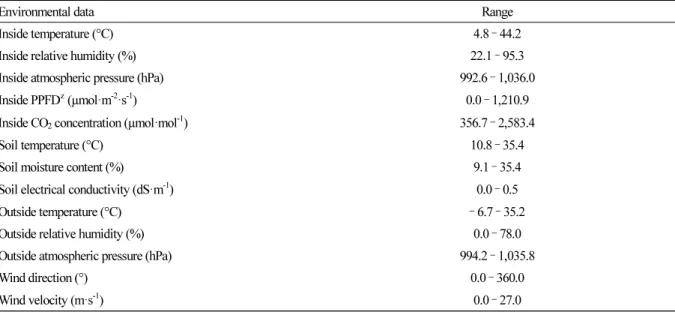
Table 1. Ranges of environmental data used as inputs of long short-term memory (LSTM). The values represent the averaged data measured by nine sensors in the greenhouse. PPFD was calculated using a conversion factor (54 lx·µmol-1·m2·s)
Environmental data Range
Inside temperature (°C) 4.8 ‑ 44.2
Inside relative humidity (%) 22.1 ‑ 95.3
Inside atmospheric pressure (hPa) 992.6 ‑ 1,036.0
Inside PPFDz (µmol·m-2·s-1) 0.0 ‑ 1,210.9
Inside CO2 concentration (µmol·mol-1) 356.7 ‑ 2,583.4
Soil temperature (°C) 10.8 ‑ 35.4
Soil moisture content (%) 9.1 ‑ 35.4
Soil electrical conductivity (dS·m-1) 0.0 ‑ 0.5
Outside temperature (°C) ‑ 6.7 ‑ 35.2
Outside relative humidity (%) 0.0 ‑ 78.0
Outside atmospheric pressure (hPa) 994.2 ‑ 1,035.8
Wind direction (°) 0.0 ‑ 360.0
Wind velocity (m·s-1) 0.0 ‑ 27.0
zPPFD, photosynthetic photon flux density.
measured illumination and converted it into photosynthetic photon flux density (PPFD) using a conversion factor (54 lx·µmol-1·m2·s). Greenhouse environmental data were measured every 10 min from February 2, 2017 to May 31, 2018.
Weather data for the same period were gathered at Boryeong Meteorological Station.
LSTM
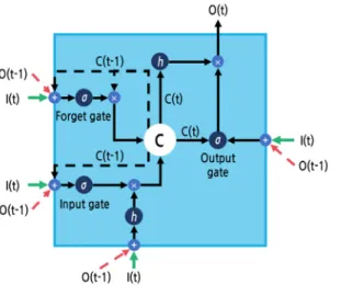
LSTM solved the vanishing gradient problem of RNNs, so LSTM can memorize long-period sequences (Hochreiter and Schmidhuber, 1997). The LSTM consists of a cell with several gates (Fig. 2). The symbols h and σ represent the input activation function and gate activation function, respectively. LSTM adds previous data to the cell state, so there is no vanishing gradient or exploding gradient problem. Computationally, LSTM accepts current input and previously processed output at the same time. The accepted values are operated at the gates. Processed information is saved in the cell state, so sequences can be memorized. Gates of LSTM are divided into three parts. The input gate determines how to select the input and output. The forget gate determines how much previous information should be forgotten. The output gate mixes the cell state with input data. LSTM yields the final output when the computation step reaches the predetermined time step.
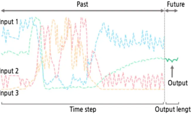
An RNN has hidden layers similar to an ordinary ANN. Input and output activation functions were set to the hyperbolic tangent function, and the gate activation function was set to the sigmoidal function. The number of perceptrons was variously combined to determine the optimal structure. In this study, previous environmental data were used as input, and the average CO2 concentration of the nine sensors was used as output. The learning rate and the time step of LSTM were varied to determine the optimal value, and the output length was set to 12 (Fig. 3). AdamOptimizer was used to train the LSTM (Kingma and Ba, 2014). The hyperparameters for the LSTM and AdamOptimizer were set to empirically used values (Table 2). For regularization, layer normalization was also used (Ba et al., 2016). Generally, neural networks are set to minimize cost (Rumelhart et al., 1988). In this study, the mean squared error (MSE) instead of the root mean squared error (RMSE) was used as a cost for reducing computation. The coefficient of determination (R2) was used for training and test accuracy. RMSE was used for verifying model robustness. TensorFlow (v. 1.12.0) was used for computation (Abadi et al., 2016).
Fig. 2. A structure of long short-term memory (LSTM). I, inputs; O, outputs; C, cell states; h, tanh activation function; σ, sigmoidal activation function; t and t-1, current and previous times, respectively.
Data Interpolation and Preprocessing
Missing data were filled using interpolation methods. Linear interpolation was used for the missing data with an interval of less than 30 min, while MLP was used for the missing data with longer intervals. Completely missing data, which cannot be inferred using other contemporary environmental factors, were filled with the data from 1 week prior. To train the LSTM, the data were normalized from 0 to 1 to improve training efficiency. The dataset was prepared according to the time step and output length. All datasets had an interval of 10 min and were periodically divided into training and test data.
To prevent the test information from being included in the training data, the training dataset did not include the period of the test dataset. That is, the datasets were divided without overlapping. In this study, the number of datasets was 69,684, and five-fold cross validation was conducted using a training and test dataset.
Results and Discussion
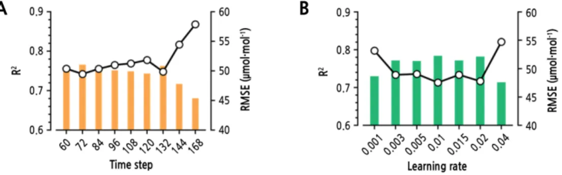
The trained LSTM showed acceptable performance in the prediction of greenhouse CO2 concentrations. In this study, the optimal time step was 72 (720 min; data interval: 10 min), and the optimal learning rate was 0.01 (Fig. 4). The test accuracies tended to decrease with the extension of the time step. Various learning rates did not change the test accuracies except 0.001 and 0.04. The LSTM is known for solving the vanishing gradient problem in recurrent neural networks (Hochreiter and Schmidhuber, 1997). In particular, the LSTM can deal with >1,000 time steps in natural language Fig. 3. A conceptual diagram of long short-term memory training. The time step varied to find the optimal value, as shown
in Fig. 4, and the output length was set to 12 with an interval of 2 h. Refer to Table 1 for details on the input factors.
Table 2. Hyperparameters for LSTM and AdamOptimizer
Parameter Value Description
β1 0.9 Exponential mass decay rate for the momentum estimates
β2 0.999 Exponential velocity decay rate for the momentum estimates
0.0001A constant for numerical stability
Dropout probability 0.1Probability of dropping out units in the neural network Forget bias 1.0 Probability of forgetting information in the previous dataset Number of perceptrons 12 The number of perceptrons used for hidden layer of LSTM and FCz
zFully connected layers.
processing (Wu et al., 2016). Therefore, the information exceeding 720 min was not meaningful for predicting greenhouse CO2 concentrations. In fact, CO2 concentrations change in a short time, so a 10-min interval could be too long for prediction (Lashof, 1989; Moon et al., 2018b). Therefore, a long time step with a short interval could yield higher accuracy.
However, the trained LSTM with a time step of 72 and a 0.01 learning rate yielded an R2 of almost 0.8, and the accuracy was higher than the previous applications of LSTM (Rußwurm and Körner, 2017; Zhang et al., 2018; Moon et al., 2019).
Since the highest accuracy was yielded with a time step of 72 and a 0.01 learning rate, subsequent experiments were conducted using the same hyperparameters.
For the validation, the average training accuracy and test accuracy of all five validations was R2 = 0.83 and 0.78, respectively (Fig. 5). The graph shows some variance, but the R2 and RMSE were adequate. The trained LSTM showed the tendency to underestimate the CO2 concentrations. CO2 concentrations in the range around 1,000 µmol·mol-1 were especially underestimated. High CO2 concentrations usually occurred when CO2 was fertilized unnaturally, so they could not be predicted using only environmental factors. More various data such as controls, workbooks, or images could increase model accuracy (Kamilaris and Prenafeta-Boldú, 2018). In this study, plant growth data were not used for investigating whether the greenhouse environment could be predicted only with environment factors. Therefore, adding plant growth can improve model robustness because the greenhouse environment is disturbed by plants. The external CO2
concentration is almost constant and may help a bit. Since the trained LSTM yielded a sequence of outputs using multiple kinds of inputs, conventional algorithms such as ARIMA models, multivariate regression, or multilayer perceptrons could not be trained in the same training condition.
A B
Fig. 4. R2 and root mean squared errors (RMSEs) of the test data at various time steps (A) and learning rates (B). Bars and solid lines represent R2 and RMSE, respectively.
A B
Fig. 5. Comparison of predicted and measured CO2 concentrations in the greenhouse for training (A) and test (B) data. The unit of RMSE is µmol·mol-1.
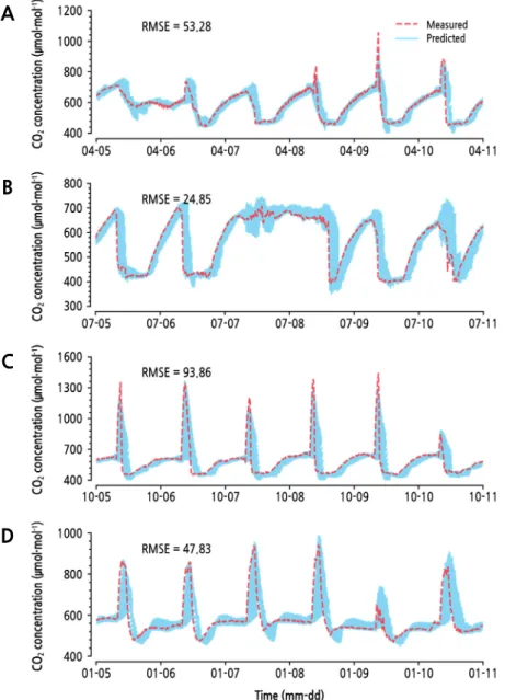
For a seasonal comparison, the LSTM showed the best accuracy from July 5 to 11, 2017 (Fig. 6). The prediction had especially high variance in autumn from October 5 to 11, 2017. Generally, the predicted area showed the possibility of underestimating fertilized CO2. In particular, a previous pattern was repeated as outputs of LSTM. One of the characteristics of LSTM is to accept previous information, so it can be seen that the previous information had a more influential effect on the prediction prior to the inference of the future changes. Therefore, some generative models could be more effective than LSTM in the case of long-term prediction (Sutskever et al., 2014; Oord et al., 2016).
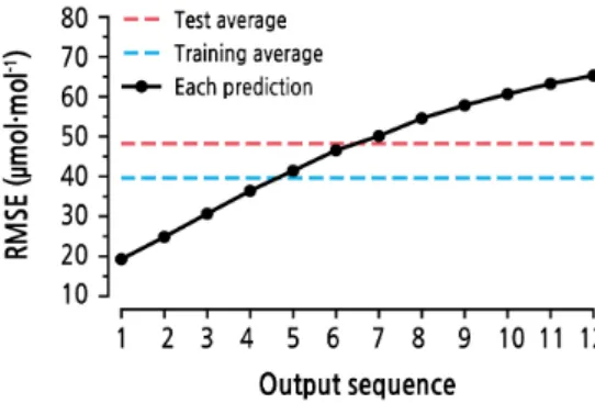
RMSEs of time-series outputs showed an increasing pattern; the lowest value was 19.257 and the highest value was 65.297 (Fig. 7). Considering the range of CO2 concentrations, the RMSEs were not high. However, the RMSE of the last output is three times higher than the first output, so another cost function would be required to conduct regression using
A
B
C
D
Fig. 6. Test of the long short-term memory by comparing measured and predicted CO2 concentrations in the greenhouse from April 5 to 11, 2017 (A), July 5 to 11, 2017 (B), October 5 to 11, 2017 (C), and January 5 to 11, 2018 (D). The unit of RMSE is µmol·mol-1 .
the LSTM (Wen et al., 2015). The costs of outputs were calculated simultaneously, so the model can only deal with the sum of the costs. To train the LSTM regressor, sequence-independent values should be studied. However, the LSTM showed adequate accuracy in prediction of CO2 concentrations, so the trained LSTM can be used to predict the future CO2
concentration and applied to efficient CO2 enrichment for photosynthesis enhancement in greenhouses. In this study, the greenhouse CO2 concentrations could be relatively well predicted. To ensure that the trained LSTM is applicable to all cultivation conditions, the model should be applied to and verified at other cultivation sites.
Literature Cited
Abadi M, Barham P, Chen J, Chen Z, Davis A, Dean J, Devin M, Ghemawat S, Irving G, et al. (2016) TensorFlow: A system for large-scale machine learning. In Proceedings of 12th USENIX OSDI, 265-283. Savanah, GA, USA, 02-04 November 2016
Ba JL, Kiros JR, Hinton GE (2016) Layer normalization. arXiv preprint arXiv:1607.06450
Boulard T, Kittas C, Roy JC, Wang S (2002) SE—structures and environment: Convective and ventilation transfers in greenhouses, part 2:
Determination of the distributed greenhouse climate. Biosyst Eng 83:129-147. doi:10.1006/bioe.2002.0114
Cock JH, Yoshida S (1973) Photosynthesis, crop growth, and respiration of a tall and short rice varieties. Soil Sci Plant Nutr 19:53-59.
doi:10.1080/00380768.1973.10432519
Davison IR (1991) Environmental effects on algal photosynthesis: Temperature. J Phycol 27:2-8. doi:10.1111/j.0022-3646.1991.00002.x Donohue RJ, Roderick ML, McVicar TR, Farquhar GD (2013) Impact of CO2 fertilization on maximum foliage cover across the globe’s
warm, arid environments. Geophys Res Lett 40:3031-3035. doi:10.1002/grl.50563
Gifford RM, Rawson HM (1994) Investigation of wild and domesticated vegetation in CO2 enriched greenhouses. In Proc. IGBP Workshop on Design and Execution of Experiments on CO2 Enrichment, Weidenberg, Germany, October 26-30, 1992
Goto E (2012) Plant production in a closed plant factory with artificial lighting. Acta Hortic 956:37-49. doi:10.17660/ActaHortic.2012.956.2 Graamans L, Baeza E, Van Den Dobbelsteen A, Tsafaras I, Stanghellini C (2018) Plant factories versus greenhouses: Comparison of
resource use efficiency. Agric Syst 160:31-43. doi:10.1016/j.agsy.2017.11.003
Greff K, Srivastava RK, Koutník J, Steunebrink BR, Schmidhuber J (2017) LSTM: A search space odyssey. IEEE Trans Neural Netw Learn Syst 28:2222-2232. doi:10.1109/TNNLS.2016.2582924
Han S, Kang J, Mao H, Hu Y, Li X, Li Y, Xie D, Luo H, Yao S, et al. (2017) ESE: Efficient speech recognition engine with sparse LSTM on FPGA. Proceedings of the 2017 ACM/SIGDA International Symposium on Field-Programmable Gate Arrays 75-84. doi:10.1145/302 0078.3021745
Hochreiter S, Schmidhuber J (1997) Long short-term memory. Neural Comput 9:1735-1780. doi:10.1162/neco.1997.9.8.1735 Hu Q, Zhang R, Zhou Y (2016) Transfer learning for short-term wind speed prediction with deep neural networks. Renew Energ 85:83-95.
doi:10.1016/j.renene.2015.06.034
Jung DH, Kim D, Yoon HI, Moon TW, Park KS, Son JE (2016) Modeling the canopy photosynthetic rate of romaine lettuce (Lactuca sativa L.) grown in a plant factory at varying CO2 concentrations and growth stages. Hortic Environ Biotechnol 57:487-492. doi:10.1007/
s13580-016-0103-z
Fig. 7. Root mean squared errors (RMSEs) of predicted CO2 concentrations in the greenhouse. RMSEs were separately calculated based on each prediction. Red and blue dashed lines represent the average RMSEs of the test and training data, respectively.
Kamilaris A, Prenafeta-Boldú FX (2018) Deep learning in agriculture: A survey. Comput Electron Agric 147:70-90. doi:10.1016/j.compag.
2018.02.016
Kaplan A, Badger MR, Berry JA (1980) Photosynthesis and the intracellular inorganic carbon pool in the bluegreen alga Anabaena variabilis: Response to external CO2 concentration. Planta 149:219-226. doi:10.1007/BF00384557
Kingma D, Ba J (2014) Adam: A method for stochastic optimization. arXiv preprint arXiv:1412.6980v9
Kläring HP, Hauschild C, Heißner A, Bar-Yosef B (2007) Model-based control of CO2 concentration in greenhouses at ambient levels increasescu cumber yield. Agric Forest Meteorol 143:208-216. doi:10.1016/j.agrformet.2006.12.002
Lashof DA (1989) The dynamic greenhouse: Feedback processes that may influence future concentrations of atmospheric trace gases and climatic change. Climatic Change 14:213-242. doi:10.1007/BF00134964
Lawlor DW (1995) Photosynthesis, productivity and environment. J Exp Bot 1449-1461. doi:10.1093/jxb/46.special_issue.1449 Linker R, Seginer I, Gutman PO (1998) Optimal CO2 control in a greenhouse modeled with neural networks. Comput Electron Agric
19:289-310. doi:10.1016/S0168-1699(98)00008-8
Liu Y, Racah E, Correa J, Khosrowshahi A, Lavers D, Kunkel K, Wehner M, Collins W (2016) Application of deep convolutional neural networks for detecting extreme weather in climate datasets. arXiv preprint arXiv:1605.01156
Lotfiomran N, Köhl M, Fromm J (2016) Interaction effect between elevated CO2 and fertilization on biomass, gas exchange and C/N ratio of European beech (Fagus sylvatica L.). Plants 5:38. doi:10.3390/plants5030038
Maroco JP, Breia E, Faria T, Pereira JS, Chaves MM (2002) Effects of long‐term exposure to elevated CO2 and N fertilization on the development of photosynthetic capacity and biomass accumulation in Quercus suber L. Plant Cell Environ 25:105-113. doi:10.1046/
j.0016-8025.2001.00800.x
McGrath JM, Lobell DB (2013) Regional disparities in the CO2 fertilization effect and implications for crop yields. Environ Res Lett 8:014054. doi:10.1088/1748-9326/8/1/014054
Mnih V, Kavukcuoglu K, Silver D, Rusu AA, Veness J, Bellemare MG, Graves A, Riedmiller M, Fidjeland, AK, et al. (2015) Human-level control through deep reinforcement learning. Nature 518:529-533. doi:10.1038/nature14236
Moon T, Ahn TI, Son JE (2018a) Forecasting root-zone electrical conductivity of nutrient solutions in closed-loop soilless cultures via a recurrent neural network using environmental and cultivation information. Front Plant Sci 9:859. doi:10.3389/fpls.2018.00859 Moon TW, Jung DH, Chang SH, Son JE (2018b) Estimation of greenhouse CO2 concentration via an artificial neural network that uses
environmental factors. Hortic Environ Biotechnol 59:45-50. doi:10.1007/s13580-018-0015-1
Moon T, Ahn TI, Son JE (2019) Long short-term memory for a model-free estimation of macronutrient ion concentrations of root-zone in closed-loop soilless cultures. Plant Methods 15:59. doi:10.1186/s13007-019-0443-7
Oechel WC, Cowles S, Grulke N, Hastings SJ, Lawrence B, Prudhomme T, Riechers G, Strain B, Tissue D, et al. (1994) Transient nature of CO2 fertilization in Arctic tundra. Nature 371:500. doi:10.1038/371500a0
Oord AVD, Dieleman S, Zen H, Simonyan K, Vinyals O, Graves A, Kalchbrenner N, Senior A, Kavukcuoglu K (2016) Wavenet: A generative model for raw audio. arXiv preprint arXiv:1609.03499
Roy JC, Boulard T, Kittas C, Wang S (2002) PA-Precision Agriculture: Convective and ventilation transfers in greenhouses, Part 1: The greenhouse considered as a perfectly stirred tank. Biosyst Eng 83:1-20. doi:10.1006/bioe.2002.0107
Rumelhart DE, Hinton GE, Williams RJ (1988) Learning representations by back-propagating errors. Cognit Model 5:1
Rußwurm M, Körner, M (2017) Multi-temporal land cover classification with long short-term memory neural networks. Int Arch Photogramm Remote Sens Spat Inf Sci 42:551. doi:10.5194/isprs-archives-XLII-1-W1-551-2017
Sharma-Natu P, Khan FA, Ghildiyal MC (1998) Photosynthetic acclimation to elevated CO2 in wheat cultivars. Photosynthetica 34:537-543.
doi:10.1023/A:1006809412319
Silver D, Huang A, Maddison CJ, Guez A, Sifre L, Van Den Driessche G, Schrittwieser J, Antonoglou I, Panneershelvam V, et al. (2016) Mastering the game of Go with deep neural networks and tree search. Nature 529:484-489. doi:10.1038/nature16961
Sutskever I, Vinyals O, Le QV (2014) Sequence to sequence learning with neural networks. In Z Ghahramani, M Welling, C Cortes, ND Lawrence, KQ Weinberger, eds, Advances in Neural Information Processing Systems, Ed 27, pp 3104-3112
Wang X, Gao L, Song J, Shen H (2017) Beyond frame-level CNN: Saliency-aware 3-D CNN with LSTM for video action recognition. IEEE Signal Process Lett 24:510-514. doi:10.1109/LSP.2016.2611485
Wen TH, Gasic M, Mrksic N, Su PH, Vandyke D, Young S (2015) Semantically conditioned LSTM-based natural language generation for spoken dialogue systems. arXiv preprint arXiv:1508.01745. doi:10.18653/v1/D15-1199
William WE, Garbutt K, Bazzaz FA, Vitousek PM (1986) The response of plants to elevated CO2. Oecologia 69:454-459. doi:10.1007/BF0 0377068
Wu Y, Schuster M, Chen Z, Le QV, Norouzi M, Macherey W, Krikun M, Cao Y, Gao Q, et al. (2016) Google’s neural machine translation system: Bridging the gap between human and machine translation. arXiv preprint arXiv:1609.08144
Zhang J, Zhu Y, Zhang X, Ye M, Yang J (2018) Developing a long short-term memory (LSTM) based model for predicting water table depth in agricultural areas. J Hydrol 561:918-929. doi:10.1016/j.jhydrol.2018.04.065
Zhao F, Feng J, Zhao J, Yang W, Yan S (2018) Robust LSTM-autoencoders for face de-occlusion in the wild. IEEE Trans Image Process 27:778-790. doi:10.1109/TIP.2017.2771408