MOVING OBJECT JOIN ALGORITHMS USING TB-TREE
Jai-Ho Lee, Seong-Ho Lee, Ju-Wan Kim
LBS Research Team, Telematics Research Group, ETRI {snoopy, sholee, juwan}@etri.re.kr
ABSTRACT:
The need for LBS (Location Based Services) is increasing due to the widespread of mobile computing devices and positioning technologies. In LBS, there are many applications that need to manage moving objects (e.g. taxies, persons).
The moving object join operation is to make pairs with spatio-temporal attribute for two sets in the moving object database system.
It is import and complicated operation. And processing time increases by geometric progression with numbers of moving objects.
Therefore efficient methods of spatio-temporal join is essential to moving object database system.
In this paper, we apply spatial join methods to moving objects join. We propose two kind of join methods with TB-Tree that preserves trajectories of moving objects. One is depth first traversal spatio-temporal join and another is breadth-first traversal spatio- temporal join. We show results of performance test with sample data sets which are created by moving object generator tool.
KEY WORDS: Moving Objects, join, TB-tree
1. INTRODUCTION
Many researchers have been studying moving object database system which manages moving objects such as vehicle on road or soldier on the battlefield. Technologies of moving object database are applied various field for example LBS(Location Baseed Service) or Telematics. The technology of Moving objects database which manages effectively moving objects getting more and more important.
We divided Research for moving objects into two parts.
One is moving objects data model and query language.
The other is index for moving objects. In this paper, we considered the mo ving point(MPoint)[4] among moving objects, because our research oriented base engine for LBS applications. We focus on query and join algorithm for past trajectory.
The spatio -temporal join operation is to make pairs with spatio-temporal attribute for two sets. It is an important type of query for multiple scanning in moving databases.
It is a sample query of spatio-temporal join : “Find all pairs of friends which distance of between two friends had been smaller than ten meter in yesterday.”
Because the spatio-temporal join requires multiple scanning, it needs large disk I/O and CPU time. Until now studying of join for moving object was in defect.
We can process join operation more effective, if two sets which are target of join operation have spatio - temporal indexes. In the paper, we consider that all two sets have spatio -temporal index. We use the TB-tree among past spatio -temporal indexes. First we overview
spatial join algorithm developed formerly, and describe how to extend it to spatio-temporal join.
2. RELATED WORKS
We classify spatial join algorithm using two spatial indexes into depth-first traversal R-tree spatial join, breadth-first traversal R-tree spatial join and transform- space view based spatial join.
The depth-first spatial join algorithm finds pairs of leaf node overlapping each other through depth-first traversing. The basic idea is to use the property that directory rectangles from minimum bounding box of ther data rectangles in the corresponding subtrees. Thus, if the rectangles of two directory entries Er and Es do not have a common intersection, there will be no pair (rectr, rects) of intersecting data rectangles where rectr is in the subtree of Er and rects is in the subtree of Es. Otherwise, there might be a pair of intersecting data rectangles in the corresponding sub trees. And local plane sweeping and pinning methods are used in order to preventing several reading to same nodes. But because heuristic methods do not consider access order of whole nodes participated in join operation and interest only access order of subtrees whose one pair of non-leaf nodes has common intersection, it’s defect is that it can’t find global optimum.
The breadth-first spatial join algorithm store pair of
nodes have a common intersection in IJI(intermediate join
index) through breadth-first searching. In IJI, since access
order of whole node is considered, global optimal join
sequences can be created. But if numbers of node pairs
have a common intersection store IJI, size of IJI increase rapidly and there is a remarkable drop in performance in contrast to depth-first traversal R-tree spatial join.
The transform-space view based spatial join order leaf nodes of one R-tree with spatial adjacency, and process region query one by one on other R-tree using ordered leaf nodes. Nodes accessed in previous query processing can be used to the highest degree in next query processing. That improves usage of buffer. Ordering leaf nodes of R-tree is achieved by space filling curve. Cost of ordering can be minimized if index is used when it is ordered. This method is proposed recent and become generally known that it shows best performance among join algorithms. But we need extension because it can only be applied in spatial index.
3. DEPTH-FIRST TB-TREE JOINS
The depth-first TB-Tree join algorithms is extended from R-tree join algorithm.
Figure 1. Structure of TB-Tree
Figure 1 is a structure of TB-tree. The TB-tree discretely extracts moving object location, represents two continuous locations of extracted moving objects as line segment, and represents set of connected line segments as trajectory. It is an access method that strictly preserves trajectories such that a leaf node only contains segments belonging to the same trajectory.
The basic algorithm of spatio-temporal join for TB-tree uses a characteristic of TB-tree strurecture that entries in nodes are sorted by time and MBB like cube. Axises of cube consist of X axis, Y axis and T(time) axis. If the MBBs of two node entrires Er and Es do not have a common intersection, there will be no pair (MBBr, MBBs).
Otherwise there might be a pair of intersecting data MBBs in the corresponding subtrees. In the follo wing subsections we assume that both trees are of the same height.
STJ1(SpatioTemporalJoin1) presents first approach based depth-first traversal approach. The TB- tree has the structual charateristic that all entries are sorted by time.
The SortedIntersectionTest function is applied plance- sweep method for intersection operation using this characteristic. It is unnecessary to sort by one axix, because nodes were already sorted. This can reduce cost.
Additionally, the local plane-sweep order with pinning method is a optimal method which reduce CPU-time and IO-time.
We restrict the search space of the join. In algorithm SpatioTemporalJoin1, each entry of the one node is checked for the join condition using the plane sweep against all entries of the other node. But before all entries of R is compared all entries of S, each entries of R is checked having a common intersection with S. each entries of S also is checked having a common intersection with R. This process can reduce considerably comparison number.
x
t R S
Figure 2. Restriction of search area.
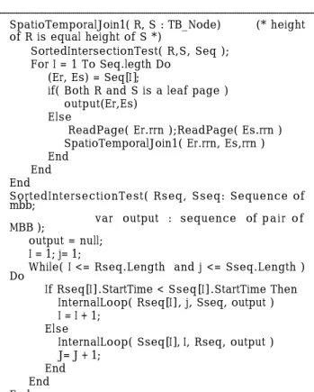
SpatioTemporalJoin1( R, S : TB_Node) (* height of R is equal height of S *)
SortedIntersectionTest( R,S, Seq );
For I = 1 To Seq.legth Do (Er, Es) = Seq[I];
if( Both R and S is a leaf page ) output(Er,Es)
Else
ReadPage( Er.rrn );ReadPage( Es.rrn ) SpatioTemporalJoin1( Er.rrn, Es,rrn ) End
End End
SortedIntersectionTest( Rseq, Sseq: Sequence of mbb;
var output : sequence of p a i r o f MBB );
output = null;
I = 1; j= 1;
While( I <= Rseq.Length and j <= Sseq.Length ) Do
If Rseq[I].StartTime < Sseq[I].StartTime Then InternalLoop( Rseq[I], j, Sseq, output ) I = I + 1;
Else
InternalLoop( Sseq[I], I, Rseq, output ) J= J + 1;
End
End
End
An example is illustrated in Figure. 2. When algorithm SpatioTemporalJoin1 performs the plane sweep, 4 segments in R area and 4 segments in S area are participated. But new algorithm SpatioTemporalJoin2 are required 3 segments in R area and 3 segments in S area.
Therefore, number of comparison required in order to compute the join condition is reduced. The modified algorithm is specified as follows.
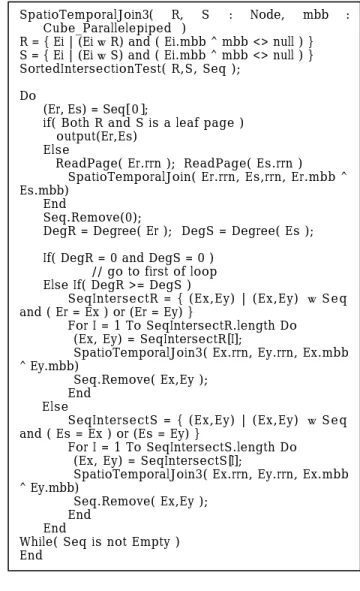
We apply “local plane-sweep order with pinning”
method to TB-tree joins. We determine a pair (Er,Es) of entries with respect to the local plane sweep order. After the corresponding subtree Er.rrn and Es.rrn, we compute degree of the cubes of both entries. The degree of an cube of entry E, short degree(E.cube) is given by the number of intersection between cube E.cube and the cubes which belong to entries of the other tree not processed util now. we pin the page in the buffer whose corresponding cube has maximal degree. The spatio- temporal join is performed on the pinned page with all other pages. Then we determine the next pair of entries using the local plane-sweep order again. In example of Figure 3, we obtain degree(R1)=0 and degree(S2)=2. Thus, the read schedule is <R1, S2, R4, R3, S1, S2>.
x
t R1
S1
R2 R3
R4 S2
S R