231
A Case Study for Simulation of a Debris Flow with DEBRIS-2D at Inje, Korea
Byung-Gon Chae1*, Ko-Fei Liu2, and Man-Il Kim3
1Geologic Environment Research Division, Korea Institute of Geoscience and Mineral Resources
2Dept. of Civil Engineering, National Taiwan University, Taiwan R.O.C.
3Office of Environmental Geology, Korea Rural Community and Agriculture Corporation
DEBRIS-2D를 이용한 인제지역 토석류 산사태 거동모사 사례 연구
채병곤1*·Ko-Fei Liu2·김만일3
1한국지질자원연구원 지구환경연구본부, 2국립대만대학교 토목공학과, 3한국농촌공사 환경지질처
In order to assess applicability of debris flow simulation on natural terrain in Korea, this study introduced the DEBRIS-2D program which had been developed by Liu and Huang (2006). For simulation of large debris flows composed of fine and coarse materials, DEBRIS-2D was developed using the constitutive relation proposed by Julien and Lan (1991). Based on the theory of DEBRIS-2D, this study selected a valley where a large debris flow was occurred on July 16th, 2006 at Deoksanri, Inje county, Korea. The simulation results show that all mass were already flowed into the stream at 10 minutes after starting. In 10minutes, the debris flow reached the first geolo- gical turn and an open area, resulting in slow velocity and changing its flow direction. After that, debris flow started accelerating again and it reached the village after 40 minutes. The maximum velocity is rather low between 1 m/sec and 2 m/sec. This is the reason why debris flow took 50 minutes to reach the village. The depth change of debris flow shows enormous effect of the valley shape. The simulated result is very similar to what happened in the field. It means that DEBRIS-2D program can be applied to the geologic and topographic conditions in Korea with- out large modification of analysis algorithm. However, it is necessary to determine optimal reference values of Korean geologic and topographic properties for more reliable simulation of debris flows.
Key words : Debris flow simulation, DEBRIS-2D, Maximum velocity, Depth change, Korean geologic and topo- graphic properties
이 연구는 Liu and Huang (2006)이 개발한 DEBRIS-2D 프로그램을 이용하여 한국의 자연사면을 대상으로 토석류 거동모사의 적용성을 평가하기 위하여 수행하였다. 세립질 및 조립질 물질이 혼재한 대규모 토석류를 모사하기 위해 DEBRIS-2D는 Julien and Lan (1991)이 제안한 구성식을 이용하여 개발되었다. DEBRIS-2D의 이론을 바탕으로 이 연구는 2006년 7월 16일 강원도 인제군 덕산리에서 대규모 토석류 산사태가 발생한 계곡을 모사대상지역으로 선택하였다. 거동 모사 결과, 토사 물질은 산사태 발생 10분 후에 이미 계곡으로 모두 유입되었다. 10분 후 토석류는 계곡부의 첫 번째 변곡점 지점인 개활지에 이르렀으며, 이로 인해 토석류의 속도가 감소하고 흐름 방향이 변하였다. 그 후 토석류는 다시 가속도가 붙어 약 40분 후에 계곡 하류의 마을인근에 이르렀다. 토석류의 최대 속도는 1 m/sec에서 2 m/sec 정도로 비교적 느리고, 토석류의 깊이변화는 계곡의 형태에 많은 영향을 받음을 알 수 있다. 거동모사 결과는 산사태 발생당시 현장의 상황과 매우 유사하게 나타났다. 이는 DEBRIS-2D 프로그램이 알고리즘을 크게 수정하지 않고도 한국의 지질 및 지형조건에 어느 정도 적용 가능함을 의미한다. 그러나, 더욱 신뢰도 높은 토석류 거동모사를 위해서는 국내 지질 및 지형에 대한 최적의 속성값을 결정할 필요가 있다.
주요어 : 토석류 거동모사, DEBRIS-2D, 최대 속도, 깊이 변화, 한국의 지질 및 지형 속성값
*Corresponding author: [email protected]
Introduction
As the world population increases and global warming effect is manifested in time, natural hazards will become the major issue all over the world. During 2005 and 2015 it had already been announced as the natural hazard prevention period by United Nation/ISDR. For countries with large portion of mountainous area, landslide and debris flows will be the major threat to residents around mountainous area. If there is no resident living in slope land area, landslides and debris flows are just natural phenomena of the earth. However, as eco- nomics grows, people have no choice but gradually moving to mountainous area. These natural phenomena then will induce hazards and cause heavy damage to those residents. How to predict the affected area and how to evaluate the economic loss from potential hazard are the key issues within the governing decision making process. One of the most effective ways of doing the assessment is to perform numerical simulations. This approach has also been the trend of the current researches as well as application to the worldwide.
Many researchers developed numerical models to simulate debris flows under different situations. Steady flow solutions with a yield stress were studied by Johnson (1970), Liu & Mei (1989), and Coussot &
Proust (1996). Liu & Mei (1989) and Ng & Mei (1994) also studied roll waves for mud flows. Huang
& Garcia (1998) studied two-dimensional slow unsteady flow from constant source and used matched-asymptotic perturbation to patch the wave front. Mei & Yuhi (2001) studied three-dimensional slow flow in elliptic channel and found dead zone within the cross section.
Iverson et al. (2000) used a two-phase flow model to simulate debris flows flowing from a large scale flume (5 m by 100 m) to a wide deposition basin. Models used for debris-flow simulation are usually depth averaged two-dimensional models. Most of the above studies focused on laboratory scale experiments or slow debris flow motion in regular channels. However, debris flows in the field have length and velocity scaled several orders larger than those in the laboratory.
Combined with the complicated geometry, the pheno-
menon in the field is quite different from a controlled environment.
O’Brien and Julien (1997) used the Julien and Lan (1991) model to simulate hyper-concentrated sediment flow and developed the commercial software FLO-2D.
FLO-2D uses 2-D kinematic equations and a central difference routing scheme. It is a dynamic routing model which does not have the capacity to deal with shock conditions. Tsai (1999) used a staggered grid scheme with Bagnold’s constitutive law to develop a numerical program but the computation of flow has to be terminated by adding total mass constraint. However, those programs that are actually used in real design or evaluation are still very rare. Since FLO-2D has been mainly used for flood, FLO-2D cannot be applied to flows with large boulders in debris flow field.
This study introduced the DEBRIS-2D program which had been developed by Liu and Huang (2003) and Liu and Huang (2006, 2009) to apply for simulation of a debris flow occurred at Deoksanri, Inje county, Korea in 2006. Based on the simulation results, this study verified the applicability of the DEBRIS-2D to the debris flows under the Korean geologic and topographic conditions.
Theoretical Background of DEBRIS-2D Program
Many researchers had developed numerical models for simulation of debris flows under various conditions.
For field simulation of debris flow, complicated program is necessary. Moreover, all the theoretical 1-D codes, steady condition only programs, and flow within fixed shaped channel should be excluded from consideration.
O’Brien and Julien (1997) used Bingham model to simulate mud flows and developed into a commercial software FLO-2D. This is the only commercially avai- lable code for debris flow, but FLO-2D is originally developed for flood. Therefore, Liu and Huang (2006) developed a two dimensional numerical program, DEBRIS-2D, to simulate large debris flows in the field.
Governing Equations
The x-axis coincides with the averaged bottom of the
channel and is inclined at an angle with respect to horizon. The y-axis is in the transverse direction and z-axis is perpendicular to both x- and y- axes. The governing equations are the continuity equation and momentum equations. The constitutive relation proposed by Julien and Lan (1991) is used in DEBRIS-2D. The original one-dimensional rheological model is extended to three-dimensional as
for τII>τ0 (1) εij> 0 for εII>ε0 (2) where tij is the stress tensor and εij is the strain rate tensor, τ0 is the yield stress, µd is the dynamic viscosity and µc is turbulent-dispersive parameter. µc
accounts for the dispersive stress effect in granular flows.
τII and εII represent the second invariant of the stress and strain rate tensor, respectively. Intuitively, this model, which includes the viscous effect and collision effect, could be used for mud flows and granular flows.
In fluid mechanics, boundary layer represents a thin layer near the physical boundary and is characterized by its strong shear effect. This layer is so thin that, if included in a numerical computation, it usually leads to unreasonable small mesh size or instability of the numerical schemes. Therefore, it is customary to separate the calculation of the main flow with its boundary layer.
This is also true in debris flows (Liu & Huang, 2003).
Here we define the bottom of the debris flow as z = B(x, y, t). The upper boundary of the thin boundary layer near the bottom is defined as z = B(x, y, t) + δ(x, y, t). Under long wave assumption, the vertical derivative for horizontal velocity is zero. Therefore,
(3)
This implies that the portion of debris flow near the free surface where the stress free condition applies is a two-dimensional plug flow, i.e. u u(z) and v v(z). Sub- stituting equation (3) into momentum equations, we obtain
(4)
(5)
(6)
With zero pressure at the free surface z = h(x, y, t), euqation (6) leads to static pressure
p =ρg cos θ(h−z) (7)
Since u and v are not functions of z, integrating continuity equation from the bottom z = B(x, y, t) + d(x, y, t) to the free surface z = h(x, y, t), we obtain in conservative form
(8)
(9)
(10)
where H = h(x, y, t)− B(x, y, t) − d(x, y, t) is the plug flow depth. The bottom erosion or deposition is neglected from equation (8). If the bottom erosion rate is large, modification must be added. Equations (8), (9) and (10) can be used to solve the three unknowns H, u and v. The real flow depth h can be found only if the boundary layer depth δ is known. But the ratio δ/h is small that neglecting δ at most induces small error. On application to field problems, 10% error is common in input data. Therefore, to the leading order approximation, we can neglect the boundary layer and solve the equations (8), (9), and (10). Thus, only the value of yield stress is needed, and simulation can be carried out with boundary layer neglected.
If debris flow starts from a stationary pile of mass, it can flow only if gravity effect and pressure gradient overcome the bottom yield stress. Therefore, the starting τij
τ0
εII
----+µd+µcεII
⎝ ⎠
⎛ ⎞εij
=
∂u
∂z
--- 0= ∂v
∂z ---
, =0
≠ ≠
∂u
∂t --- u u∂
∂x --- v∂u
∂y ---
+ + 1
ρ---∂p
∂x
--- gsinθ 1 ρ--- ∂τzx
∂z ---
⎝ ⎠
⎛ ⎞
+ +
–
=
∂v
∂t --- u v∂
∂x --- v v∂
∂y ---
+ + 1
ρ---∂p
∂y --- 1
ρ--- ∂τzy
∂z ---
⎝ ⎠
⎛ ⎞
+ –
=
0 1· ρ---∂p
∂z --- – –gcosθ
=
∂H
∂t --- ∂( )uH
∂x
--- ∂( )vH
∂y ---
+ + =0
( )uH
∂
∂t
--- ∂(u2H)
∂x
--- ∂(uvH)
∂y ---
+ +
g θH∂B
∂x
--- g θH∂H
∂x
--- gsinθH 1 ρ--- τ0u
u2+v2 --- – cos +
cos – –
=
( )vH
∂
∂t
--- ∂(uvH)
∂x
--- ∂(v2H)
∂y ---
+ +
g θH∂B
∂y
--- g θH∂H
∂y --- 1
ρ--- τ0v u2+v2 --- cos –
cos – –
=
condition can be obtained by setting all velocities zero in equations (9) and (10) to reach
(11)
If a one-dimensional debris pile is everywhere on the threshold of motion, the profile of the pile can be obtained by replacing greater sign by equal sign in equation (11) and integrating in x to get
(12)
This equation is used in the laboratory to determine the yield stress of any field material. A pile of field sample is slowly pushed from the upstream by a vertical plate in a flume. The resulting profile is measured and the yield stress is fitted with equation (12) as in Fig. 1.
We use Adams-Bathforth third order scheme in time and central difference and upwind scheme in space.
Upwind method is used for convective terms, while central difference is used for all other terms. Mathe- matically, one condition for H, u and v each in physical boundary is needed. For debris flows simulation in the field, it is usually necessary to find a computational domain, which contains the whole reach of the debris flows. In this case, we can use
H = 0, u = 0, v = 0 on all boundaries (13) If debris flows are restrained in a fixed domain such as in a flume, we use no normal flux condition on all physical boundaries. But equation (11) still applies to the
front and tail of the debris flows. The tracking of the points with velocity near zero is important. Correction of overshooting of physical quantities are performed every time step.
Verification of the numerical scheme
Verification with the final deposit profile
Under slow mud motion, the analytical solutions for the final profile of debris flow can be obtained (Liu and Huang, 1996). The final profile for one-dimensional flow is
(14)
This result is the same as in Liu & Mei (1989). The initial profile is a triangular pile against left wall (x = 0).
The final profile is compared with analytical results (dotted line in Fig. 2). With x = 0.1, the maximum error is 1%.
For two-dimensional flow, analytical solution with the help of the method of characteristic is also possible (Liu and Huang, 1996). An initial hump with the shape
∂h
∂x ---–tanθ
⎝ ⎠
⎛ ⎞2 ∂h
∂y ---
⎝ ⎠⎛ ⎞2
+ τ02
ρ2g2cos2(θH2) ---
>
h τ0
ρg θsin
--- h τ0
ρg θsin ---
⎝ – ⎠
⎛ ⎞
ln
+ =tanθH C+
H2 2τ0L ρgD22
---x cons tant+
⎝ ⎠
⎛ ⎞
±
=
Fig. 1. Measurement of a yield stress with equation (12) (after Liu and Huang, 2009).
Fig. 2. The comparison between numerical and analytic solutions for final depth of 1-D flow (after Liu and Huang, 2009).
H = 0.5− (x − 1.5)2− (y − 1.5)2 (15) is used. The comparison between numerical result and analytical result at the central cross-section is plotted in Fig. 3. With x = y = 0.01 and t = 0.001 the max error is 1%.
Field verification at Shen-Mu village in Nan-Tou County, Taiwan
Shen-Mu village is located within Nan-Tou county, Taiwan. Serious debris flows occurred on July 31th, 1996 during Typhoon Herb. The area is a part of Hsu-Sui river basin. River length is roughly 5 Km and the average bottom slope is 11.5 degrees. The topographic contour is plotted in Fig. 4. The deposition material is mostly clayey sand. According to the investigation by Disaster Prevention Research Center of National Cheng- Kung University, Taiwan, the volume of the total debris flows deposited is about 560,000 m3 and the dry specific gravity is 1.3. In order to simulate the flow, we distributed the total 560,000 m3 debris volume over the upstream area as in Fig. 5. Computation grid size is 10 m by 10 m, the maximum elevation difference within this area is 300 m. The yield stress is measured in situ as well as from laboratory experiments with field sample
by equation (14). The obtained value for the yield stress is roughly 1,000 N/m2. The time step used in com- putation is 0.1 sec.
The calculated final deposition profile is plotted in Fig. 6. The solid lines indicate the deposition boundary measured after the disaster. Depth contours are numeri- cally calculated results and the distribution is very close to the measured result. The only difference is at 2,300 m downstream and there is a tributary merging into the main river from top of the figure and it stopped debris flows from going into the tributary. However, in our simulation, no inflow is assigned at the merging point, therefore, debris flow can flow into the tributary where the elevation is low. Lastly, we compared the calculated height of final deposition with measured along the cross section marked by the solid line in Fig. 4. The computed result is also very close to field measurements as in Fig. 7. The local maximum difference is less than 1 m.
Fig. 3. The comparison between numerical and analytic solutions of debris flow final depth at the central cross- section for 2-D pile initially described by equation (14) (after Liu and Huang, 2009).
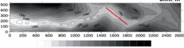
Fig. 4. The topographic contour map of Shen-Mu village.
The straight line is the cross-section where calculated depth is compared with measured final deposition depth in Fig. 7 (after Liu and Huang, 2006).
Fig. 5. The initial distribution of debris volume in the numerical model. Contour means thickness of debris (after Liu and Huang, 2006).
Fig. 6. The comparison of simulated and measured boundary of debris flow. Contour means thickness of debris (after Liu and Huang, 2006).
Fig. 7. The comparison of simulated and measured depth for final debris flow deposition along the solid line in Fig. 4 (after Liu and Huang, 2009).
Application of DEBRIS-2D to a Debris Flow at Deoksanri site, Korea
Description of the study area
Based on the theory of DEBRIS-2D, this study applied it to a debris flow in Korea to assess its appli- cability in Korean geologic and topographic condition.
The study selected a valley where a large debris flow was occurred in July 16th, 2006 at Deoksanri, Inje county, Korea. When the debris flow was occurred, the whole area of the valley in Fig. 8 was covered by huge amount of debris.
The area is composed of mountainous topography, which occupies 80% of the total area. The highest elevation around the study area reaches 945 m and the most dominant elevation distribution is grouped between 351 m and 420 m as 20.6% at the area (Fig. 9a). The
study area has relatively steep slope angles, which the highest distribution percentage of slope angle is between 31 degrees and 40 degrees as 39.6 % (Figs. 9(b) and (c)). The high elevation, steep slope angles and long
Fig. 8. Aerial photograph showing the location of simulated valley for the simulation at Deoksanri site, Korea.
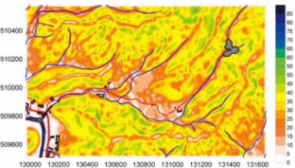
Fig. 9. Topographic characteristics of the study area and location of the landslide monitoring sensors at Deoksanri site, Inje. (a) Elevation map around the study area and the distribution of monitoring sensors at the monitoring valley, (b) Distribution of topographic elevation in the area of Fig. 9(a), (c) Distribution of slope angle in the area of Fig. 9(a).
persistence of valleys of the area have high potential to occur many landslides and long run-out distance of debris flows. Orientation of major stream is WNW- ENE and the landslide monitoring site is located along a valley of NE-SW direction.
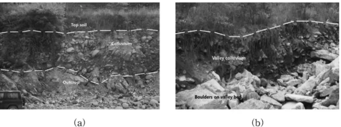
The lithology of the study area is composed of Pre- Cambrian granitic gneiss with high density of foliations and shear fractures due to complex metamorphism. The area has thick colluvium, averaging 4 m thick near the bottom of mountain and 0.5 m-2 m thick at the top and middle of it (Fig. 10). The profile of weathered soil layer on the mountain slope shows typical colluvium feature composed of loosely compacted angular rock fragments with poor sorting and sandy silt particles. The soil is uni- formly moist from top to bottom of the layer implying high permeability coefficient in the soil layer. The domi- nant size of boulders along the bed of valley is 60 cm × 50 cm induced by high density of shear fractures. This feature clearly indicates that the soil layer is material of old landslides and there have been many events of landslides and debris flows at the study area. Table 1 shows physical property of the soil at the study area.
According to Korea Meteorological Administration (KMA), the accumulated rainfall from July 15 to 20, 2007 reached about 474 mm at Inje county. Daily maximum rainfall and hourly maximum rainfall were 227 mm and 62 mm on July 15 at the area, respectively.
It is rare to record the heavy rainfall intensity and amount in this area with an annual average of 1200 mm-1500 mm. Therefore, severe debris flows were
occurred and many roads and houses are destroyed (KIGAM, 2008).
After the field survey, the following information for simulation were collected. The triggering points of landslides are about 50 points along the simulated valley.
Average length and depth of landslide are 48 m and 3 m, respectively. Slope angles of the area are distributed between 25 and 35 degrees. Because the debris flow in the simulated valley was joined a river which runs across Deoksanri village, this study designated the final spread position at the junction between the simulated
Fig. 10. Depositional features of colluviums and large boulders at the bottom of mountain (a) and at the middle of mountain (b) in the study area.
Table 1. Soil physical properties of the model slopes for the flume tests
Property Value
Specific gravity 2.64
Moisture content (%) 14.58
Void ratio 0.69
Porosity (%) 40.97
Soil conductivity (cm/sec) 3.819×10⁻³
Density (t/m3)
Bulk density 1.82
Saturation density 1.97
Dry density 1.56
Atterberg limits
Liquid limit 30.45
Plastic limit 24.75 Plasticity index 5.70
Uniformity coefficient 10.0
Curvature coefficient 1.3
USCS SW
valley and the river. We measured the coordinates of final spread position, height and width of debris flow at the final spread position.
Simulation result using the DEBRIS-2D
Input parameters for the debris flow simulation using the DEBRIS-2D are listed in Table 2. Major categories of the input parameter are topography, source information of debris, and physical parameter of materials. The para- meters can be acquired by analysis of topography, field survey and laboratory test.
There are three locations of landslides at the upstream in the simulated valley. The accumulated regolith majorly composed of gravels and sands in the stream became debris flow during heavy rainfall. The mass distribution is listed in Table 3. Due to the abundance of gravel and sands, yield stress in this site is estimated to be 1,000 dyne/cm2 (Liu and Hwang, 2003). The area of the simulated valley is 5.5 Km2. The slope angle for initial mass area is averaged between 30 and 40 degrees. The average slope angle near the final spread position is between 10 and 20 degrees as shown in Fig. 11.
Because the resolution of digital topographic map (DTM) is 5 m×5 m, the grid size in simulation is 10 m × 10 m. We distributed 11,533 m3 of debris volume at the three initial positions of landslides (Fig. 12). Although the area is characterized to have steep slope on side
slope of streams, the stream itself flows along very mild bottom slope. This implies the velocity of debris flows will not be very high.
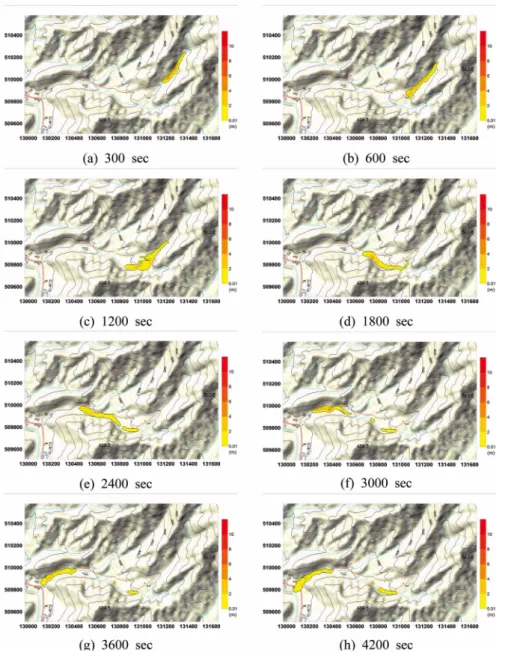
The simulation results are shown in Fig. 13. It shows the result from 5 minutes after debris flow started to 70 minutes after debris flow started. It can be seen that all mass were already flowed into the stream at 10 minutes after starting. In 10 minutes, the debris flow reached the first geological turn and an open area, resulting in slow velocity and changing its flow direction. After that, debris flow started accelerating again and it reached the village after 40 minutes.
The maximum velocity and maximum depth change are shown in Figs. 14 and 15. The maximum velocity is rather low between 1 m/sec and 2 m/sec. This is the reason why debris flow took 50 minutes to reach village. However, the depth change shows enormous effect of the valley shape. Whenever there is changes of valley widths, debris flow tends to accumulate the Table 2. Input parameters for the DEBRIS-2D
Category Parameter
Topography Elevation, Slope aspect, Slope angle, etc Source information Coordinates of source area Physical parameter Yield stress, Flow rate, Concentration time
Model parameter Computation time Ouput location Coordinates of output location
Table 3. Information of mass distribution at the three landslides positions near upstream of the target valley
E coordintae N coordinate Volume (m3)
Area (m2)
depth (m) 131395.0000 510326.5819 4360 2179.8783 2 131457.8871 510264.9525 3504 1751.9705 2 131401.2888 510239.7977 3669 1834.7483 2
Fig. 11. Slope angle distribution at the study area. The scale on the right has unit of degree. Blue curves indicate the centerline of streams. Black area on the upper right is the initial mass location.
Fig. 12. Distribution of initial mass depth at the three landslides positions listed in Table 3.
Fig. 13. Flow thickness of each 600 seconds along the simulated valley (from 300th steps to 6000th steps).
Fig. 15. Temporal variation of maximum depth for the debris flow.
Fig. 14. Temporal variation of maximum velocity for the debris flow.
mass at the front of concave region. Only after the mass accumulates high enough, the flow will accelerate again to downstream. Debris flow occurred around 9, 40 and 72 minutes after it started. Since the maximum height of the debris flow remains higher than 2.5 m, debris flows will cause total destruction of all facilities and vegetation throughout its passage.
Besides understanding the maximum height, it is
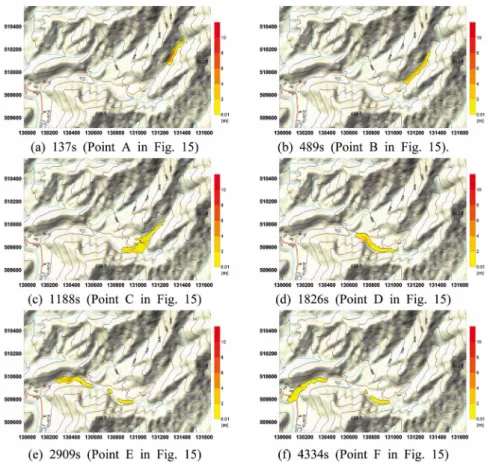
important to know when and where is the maximum height. The red area is where debris flow height exceeds 5 m (Fig. 16). It is possible to understand that the maximum height occurs near the front flow (Fig. 16 (a) and (b)), adjacent to turning point (Fig. 16(c) and (d)) and around houses (Fig. 16(e) and (f)).
The simulated result is very similar to what happened in the field (Fig. 17). Even the houses affected by the
Fig. 16. Depth distribution of debris along the simulated valley.
Fig. 17. Features of deposited debris and damages at the final spread position in the simulated valley.
debris flow in the simulation show similar damages observed in the field. It means that DEBRIS-2D pro- gram can be applied to the geologic and topographic conditions in Korea without large modification of ana- lysis algorithm. However, this study is a result of flow simulation of debris in the gneiss area. If the simula- tion method is applied to other geologic conditions, there might be different simulation results and reliability com- pared with the gneissic rocks area. Therefore, it is nece- ssary to determine optimal reference values of Korean geologic and topographic properties for more reliable simulation of debris flows. Because the purpose of the debris flow simulation is to predict potential damage area by landslides, accurate property of input parameters should be evaluated before simulation.
Conclusion
This study introduced the DEBRIS-2D program which had been developed by Liu and Huang (2006) to apply for simulation of a debris flow occurred at Deoksanri, Inje county, Korea in 2006. For simulation of large debris flows composed of fine and coarse materials, DEBRIS-2D was developed using the constitutive relation proposed by Julien and Lan (1991). Based on the theory of DEBRIS-2D, this study applied it to a simulated valley where a debris flow occurred. The simulation results show that all mass were already flowed into the stream at 10 minutes after starting. In 10 minutes, the debris flow reached the first geological turn and an open area, resulting in slow velocity and changing its flow direction. After that, debris flow started accelerating again and it reached the village after 40 minutes. The maximum velocity is rather low between 1 m/sec and 2 m/sec. This is the reason why debris flow took 50 minutes to reach village.
The depth change shows enormous effect of the valley shape. The simulated result is very similar to what happened in the field. It means that DEBRIS-2D program can be applied to the geologic and topographic conditions in Korea without large modification of analysis algorithm. However, it is necessary to determine optimal reference values of Korean geologic and
topographic properties for more reliable simulation of debris flows.
Acknowledgement
This research was supported by the Basic Research Project of the Korea Institute of Geoscience and Mineral Resources (KIGAM) funded by the Ministry of Kno- wledge Economy of Korea.
References
Coussot, P. and Proust, S., 1996, Slow, unconfined spreading of a mud flow, Journal of Geophysical Research, 101, 25217-25229.
Huang X., and Garcia, M.H., 1998, A Herschal-Hulkley model for mud flow down a slope., Journal of Fluid Mechanics, 374, 305-333.
Iverson, R.M., Denlinger, R.P., LaHusen, R.G., and Logan, M., 2000, Two-phase debris flow across 3-D terrain: Model predictions and experimental tests, in Debris-Flow Hazards Mitigation: Mechanics, Pre- diction, and Assessment G.F. Wieczorek and N.D.
Naeser, eds., Balkema, Rotterdam, 521-529.
Johnson, A.M., 1970, Physical processes in geology.
New York, 577p.
Julien, P.Y. and Lan, Y., 1991, Rheology of hypercon- centrations, Journal of Hydr. Engrg., ASCE, 117, 346-353.
KIGAM, 2008, Development of landslide prediction technology and damage mitigation countermeasures, NEMA, NEMA-06-NH-04, 566p.
Liu, K.F. and Huang, M.C., 2006, Numerical simulation of debris flow with application on hazard area map- ping, Computational Geosciences, 10, 221-240.
Liu, K.F. and Huang, M.C., 2009, Numerical Simulation of Debris Flows, Proceedings of the ASME 2009 28th International Conference on Ocean, Offshore and Arctic Engineering (OMAE2009), May 31 - June 5, 2009, Honolulu, Hawaii, USA, OMAE2009-79197.
Liu, K.F. and Huang, M.T., 1996, Study of the front shape of 3-D stationary debris flow, Proceedings of Eight Civil and Hydraulic conference, 529-536.
Liu, K.F. and Huang, M.T., 2003, Three-dimensional numerical simulation of debris flows and its appli- cations, The 3rd international conference on debris- flow hazards mitigation, 469-481.
Liu. K.F. and Mei, C.C., 1989, Slow spreading of a sheet of Bingham flulid on an inclined plane, Journal of Fluid Mechanics, 209, 505-529.
Mei, C.C. and Yuhi, M., 2001, Slow flow of a Bingham fluid in a shallow channel of finite width, Journal of Fluid Mechanics, 431, 135-159.
Ng, C. and Mei, C.C., 1994, Roll waves on a shallow layer of mud modeled as a power-law fluid, Journal of
Fluid Mechanics, 263, 151-183.
O'Brien, J.S. and Julien, P.Y., 1997, On the importance of mudflow routing, Proceedings of the 2nd International Conference on Debris Flow Hazards Mitigation, Taipei, 677-686.
Tasi, Y.F., 1999, Study on the configuration of debris flow fan, Ph.D. dissertation, National Cheng-Kung University, Taiwan, 255p.
2010년 6월 1일 원고접수, 2010년 9월 5일 게재승인 채병곤
한국지질자원연구원 지구환경연구본부 350-350 대전광역시 유성구 과학로 92 Tel: 042-868-3052
Fax: 042-868-3414 E-mail: [email protected]
Ko-Fei Liu
Department of Civil Engineering, National Taiwan University
No. 1, Sec. 4, Roosevelt Road, Taipei, 10617 Taiwan(R.O.C.)
Tel: 042-868-3052
E-mail: [email protected]
김만일
한국농어촌공사 환경지질처 437-703 경기도 의왕시 포일동 487 E-mail: [email protected]