Restoration Modeling Analysis for Abandoned Channels of the Mangyeong River
Jaehoon Kim, Pierre Y. Julien, Un Ji 1)* , Joongu Kang 2)
Department of Civil and Environmental Engineering, Colorado State University, Ft. Collins, CO 80523, USA
1) Department of Civil and Environmental Engineering, Myongji University, Yongin 449-728, Korea
2) Department of Water Resources Research, Korea Institute of Construction Technology, Ilsan 411-712, Korea (Manuscript received 7 October, 2010; revised 17 February, 2011; accepted 11 March, 2011)
Abstract
This study examines the potential restoration of abandoned channels of the Mangyeong River in South Korea. To analyze the morphological changes and equilibrium conditions, a flow duration analysis was performed to obtain the discharge of 255 m3/s with a recurrence interval of 1.5 year. It is a gravel-bed stream with a median bed diameter of 36 mm. The reach-averaged results using HEC-RAS showed that the top width is 244 m, the mean flow depth is 1.11 m, the width/depth ratio is very high at 277, the channel velocity is 1.18 m/s, and the Froude number is also high at 0.42. The hydraulic parameters vary in the vicinity of the three sills which control the bed elevation. The total sediment load is 6,500 tons per day and the equivalent sediment concentration is 240 mg/l. The Engelund-Hansen method was closer to the field measurements than any other method. The bed material coarser than 33 mm will not move. The methods of Julien-Wargadalam and Lacey gave an equilibrium channel width of 83 m and 77 m respectively, which demonstrates that the Mangyeong River is currently very wide and shallow. The planform geometry for the Mangyeong River is definitely straight with a sinuosity as low as 1.03. The thalweg and mean bed elevation profiles were analyzed using field measurements in 1976, 1993 and 2009. The measured profiles indicated that the channel has degraded about 2 m since 1976. The coarse gravel material and large width-depth ratio increase the stability of the bed material in this reach.
Key Words : Abandoned channel, Equilibrium channel width, Stream restoration, Stream morphology
1)
1. Introduction
There is an increase in environmental concerns about rivers and streams in South Korea. Mangyeong River is one of the main watersheds on the western central region of South Korea. When Mangyeong River was channelized in the early 1900’s, an abandoned channel was formed. There is interest to restore this abandoned channel to increase flow interaction, to improve water quality, to enhance
*
Corresponding author : Un Ji, Department of Civil and Environmental Engineering, Myongji University, Yongin 449-728, KoreaPhone: +82-31-330-6808 E-mail: [email protected]
wildlife habitat, and to provide an environmental friendly site for local people. This study will be used to aid in reconnecting the abandoned channel to the main river.
Restoration can have many different meaning based on the context. In most cases restoration is defined as returning to a pre-disturbance physical state (Burchsted, 2006). While, Wohl et al. (2004) define river restoration as assisting the recovery of ecological integrity in a degraded watershed system by reestablishing hydrologic, geomorphic, and ecological processes, and replacing lost, damages or compromised biological elements.
The objectives of this project are to analyze the
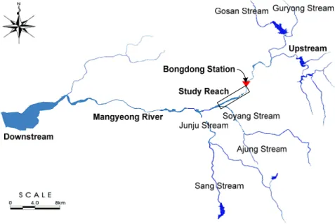
Fig. 1. Study Site Map for Mangyeong River.
morphological changes and equilibrium conditions along Mangyeong River for future abandoned channel restoration. This article reports on the following analyses: (1) a hydrologic analysis using flow duration analysis; (2) a hydraulic analysis based on HEC-RAS data; (3) a bed material classification and sediment transport capacity analysis; (4) a river equilibrium analysis using downstream hydraulic geometry; and (5) a geomorphic characterizations of the study reach using survey data and aerial photos.
2. Site Description
Mangyeong River is placed in the lower part of Kum River watershed. Mangyeong River has watershed area of 1,527 km 2 , is 77.4 km long, and is located in the following provinces: Wanju-gun, Jeonju-si, Iksan-si, Gimje-si, and Gunsan-si in Jeollabuk-do.
The study site is located just upstream of Soyang Stream tributary in Guman-ri, Bongdong-eup, Wanju-gun, Jeollabuk-do (Fig. 1). An abandoned
channel was located from Bongdong Bridge (104+
000) to upstream of Soyang Stream tributary (87+000) and its length is 4.25 km. Three sills which are Sill A (Gumanri-bo), Sill B (Sae-bo), Sill C (Jangja-bo) were constructed in 1969, 1966, and 1976 respectively.
3. Hydraulic Analysis
3.1. Flow Duration Analysis
The flow duration curve (Fig. 2) was obtained from Bongdong station which is 2km upstream of study reach. Data were available from 2004 to 2009.
A flow discharge of 255 m 3 /s corresponds to a
recurrence interval of 1.5 year from flow duration
curve shown on the flow duration curve. This
discharge is used as a reference value representing
the channel forming discharge in the foregoing
analyses of hydraulic parameters, sediment transport,
river equilibrium, and stream classification. Many
researchers recommended 1 to 5 year recurrence
interval discharge as a channel forming discharge. In this
0.01 0.1 1 10 100 1000 10000
0.1 1 10 100
PDF (%)
Q (cms)
Fig. 2. Flow Duration Curve.
study, the 1.5 year recurrence interval discharge recommended by Leopold et al. (1964), Leopold (1994), and Hey (1975) was adopted as a channel forming discharge.
3.2. HEC-RAS Modeling Analysis
The hydraulic analysis was conducted using HEC-RAS. The Manning’s n value of 0.03 is assumed based on initial observations by the surveying team.
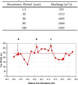
The hydraulic analysis was conducted on Mangyeong River at 5 distinct flow rates shown in Table 1.
The spatial distribution of several hydraulic parameters was examined over the study reach. These parameters include the top width (Fig. 3), wetted perimeter, maximum flow depth, cross-sectional area, mean flow depth, width/depth ratio, channel velocity, Froude number. These parameters were also determined at the channel forming discharge of 255 m 3 /s. On the Figure, the letters A, B, and C represent the three sills from upstream to downstream within study reach.
The average values of each hydraulic parameter are as follows: the top width is 239 m, the wetted perimeter is 240 m, the maximum flow depth is 1.90 m, the cross sectional area is 265 m 2 , the mean flow depth is 1.11 m, the width/depth ratio is 277, the channel velocity is 1.18 m/s, and Froude number is 0.42. These values indicate that the river is currently very wide and shallow and the Froude number is relatively high.
Table 1. Flow Rates of Different Recurrence Period of
Mangyeong RiverRecurrence Period (year) Discharge (m
3/s)
1.5 255
30 1513
50 1695
80 1864
100 1943
0 50 100 150 200 250 300 350
39.5 40.0 40.5 41.0 41.5 42.0 42.5 43.0 43.5 44.0 44.5
Distance from Downstream (km)
To p W idt h ( m )
A B C
Fig. 3. Spatial Trends of Top Width.
All results showed that there was sudden change in the location of sills. The decrease in top width, wetted perimeter, and cross sectional area at the river distance of 43 km is attributed to the agricultural development on floodplain near the left bank of Mangyeong River. The floodplain area is covers approximately 0.1 km 2 and a levee was constructed to protect agriculture area.
4. Sediment Transport
4.1. Bed Material
Samples of the bed material were taken on July 2009 and spaced 10 m apart along one cross section of Bongdong Station. The median grain size of the bed material was found to be 36 mm, which represents very coarse gravel. This coarse bed material is not very mobile and the analysis of the maximum grain diameter determines its mobility.
4.2. Maximum Movable Grain Size
From the sediment grain size, the shear stress
analysis on particle size was performed to obtain the particle size at incipient motion (Julien, 2010). The maximum moving particle size can be calculated from the following equation when the Shields parameter is critical ( c ),
( ) c
f
s G
S d R
1 τ *
= −
(1)
Where, G is the specific gravity of the sediment, R is the hydraulic radius and S
fis the friction slope.
The particle size that corresponds to incipient motion at c is 0.05 is obtained as d is 40 mm for this s study reach. The discharge with the recurrence interval of 1.5 year was selected to get hydraulic radius R from HEC-RAS and the slope S f of 0.00230 m/m from survey data. Based on the critical Shields parameter equation, the maximum movable particle size can be computed directly. The maximum movable particle size is around 33 mm (very coarse gravel). This result indicates that the sediment currently at study reach in Mangyeong River will not move until the discharge is greater than 255 m 3 /s.
4.3. Sediment Transport
The model HEC-RAS calculates sediment transport capacity using several different methods including those developed by Ackers & White, Engelund & Hansen, Laursen, Meyer-Peter & Müller, Toffaleti, and Yang (gravel). HEC-RAS results were compared with the results of sediment measurements in Bongdong Station.
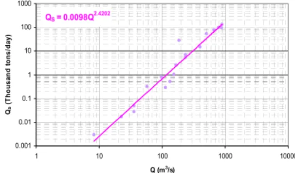
Sediment measurements were taken in July 2009 at Bongdong Station (Yongbong Bridge) in Mangyeong River from KICT (2009). From the measurements, the relationship between discharge and total sediment load was determined as shown in Fig. 4 When the channel forming discharge of 255 m 3 /s is applied, the total load is 6.54 thousand tons per day. This is
equivalent to a sediment concentration of 240 mg/l at 255 m 3 /s.
Q
S= 0.0098Q
2.42020.001 0.01 0.1 1 10 100 1000
1 10 100 1000 10000
Q (m3/s)
Qs (Thousand tons/day)
Fig. 4. Relationship between Discharge and Total Load.
Fig. 5. Sediment Rating Curve at the Cross Section 96.
With the above relationship, HEC-RAS was used
to calculate the sediment transport capacity for all six
methods at all five discharges. Only the Engelund-
Hansen method was close to measured data shown in
Fig. 5. The methods of Ackers & White and Meyer-
Peter & Müller were removed from the analysis
because the results were close to zero. The sediment
transport measurements include both the bed material
load as well as the washload (Julien, 2010). Sediment
transport formulas including the suspended load
proved to be a lot closer to the total load from the
field measurements than any other method. At a
discharge of 255 m 3 /s, the field measurements were
relatively close to the results predicted from the
method of Engelund-Hansen. Nevertheless, the
measured sediment load at higher discharges remained about 10 times larger than the calculations from the method of Engelund-Hansen. Therefore, the calculations should be based on the field measurements.
5. River Equilibrium
5.1. Equilibrium Analysis
Several hydraulic geometry equations were used to determine the equilibrium channel width. These methods use channel characteristics such as channel width and slope, sediment concentration, and discharge.
Julien and Wargadalam (1995) used the concepts of resistance, sediment transport, continuity, and secondary flow to develop semi-theoretical hydraulic geometry equations.
m m m m
d
sS Q
h
561 6 5
6 6 5
2
2 .
0 +
− +
= +
(2)
m m m m m s m
S d Q
W
562 1 6 5
4 6 5
4 2
33 .
1 ++ −+ −+−
=
(3)
m m m m m s m
S d Q
V
562 2 6 5
2 6 5
2 1
76 .
3 ++ −+ ++
=
(4)
m m s m
m
d S
Q
566 4 6 5
5 6 5
2
*=0.121 + +− ++
τ (5)
4 6
5 6 4 * 6
5 2 3
1
4 .
12 +
+ + +
−
= m
m sm
m
d
Q
S τ (6)
⎟⎟⎠
⎜⎜ ⎞
⎝
= ⎛
50
2 . ln 12
1
d m h
(7)
Where h (m) is the average depth, W (m) is the average width, V (m/s) is the average one-dimensional velocity, and τ * is the Shields parameter, and d
50(m) is the median grain size diameter.
Simons and Albertson (1963) used five sets of data from canals in India and America to develop equations to determine equilibrium channel width.
Blench (1957) used flume data to develop regime
equations. A bed and a side factor ( F s ) were developed to account for differences in bed and bank material.
(
1 0.012)
1/2 1/4 1/26 .
9
d Q
F W c
s ⎟⎟⎠
⎜⎜ ⎞
⎝
⎛ +
=
(8)
Where, W (ft) is channel width, c (ppm) is the sediment load concentration, d (mm) is the median grain diameter, and Q (ft 3 /s) is the discharge. The side factor, F s =0.1 for slight bank cohesiveness.
Lacey (from Wargadalam 1993) developed a power relationship for determining wetted perimeter based on discharge.
5 .
667 0
.
2
Q
P = (9)
Where P (ft) is wetted perimeter and Q (ft 3 /s) is discharge. For wide, shallow channels, the wetted perimeter is approximately equal to the width.
Klaassen and Vermeer (1988) used data from the Jamuna River in Bangladesh to develop a width relationship for braided rivers.
53 .
1 0
.
W =
16 Q(10)
Where W (m) is width, and Q (m 3 /s) is discharge.
Nouh (1988) developed regime equations based on data collected in extremely arid regions of south and southwest Saudi Arabia.
( )
0.93 1.2583 . 0
50 0.018 1
83 .
2
d c
Q
W Q
⎟⎟ + +⎠
⎜⎜ ⎞
⎝
= ⎛
(11)
Where W (m) is channel width, Q
50(m 3 /s) is the
peak discharge for a 50 year recurrence period, Q
(m 3 /s) is annual mean discharge, d (mm) is mean
grain diameter, and c (kg/m 3 ) is mean suspended
sediment concentration.
The results of different methods are presented in Fig. 6. The methods of Lacey and Julien and Wargadalam tend to under predict the channel width compared to main channel width. This suggests that the channel was most likely designed to carry large floods. The Simons and Albertson method tends to predict the channel widths determined from HEC-RAS at lower flows. The method of Klaassen and Vermeer tends to completely overestimate the channel width. The equations of Julien-Wargadalam and Lacey predict similar equilibrium channel widths.
Fig. 6. Predicted and Actual Width.
5.2. Stable Channel Design
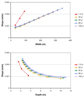
The analysis of stable channel design can be performed using the SAM Hydraulic Design Package. The stable channel design functions are based on the methods developed by the U.S. Army Corps of Engineers at the Waterways Experiment Station. In this study only the Copeland method was used. It is based on an analytical approach to solve stable channel design based on the depth, width, and slope (Fig. 7).
In summary, the sills of Mangyeong River force the river to be a lot wider and shallower than predicted with downstream hydraulic geometry relationship. Also, the fact that the riverbed is armored makes the comparisons with methods developed for alluvial rivers difficult to apply.
0 0.001 0.002 0.003
0 100 200 300 400
Width (m)
Slope (m/m) 1.5 yr
30 yr 50 yr 80 yr 100 yr
0 0.001 0.002 0.003
0 2 4 6 8 10 12
Depth (m)
Slope (m/m) 1.5 yr
30 yr 50 yr 80 yr 100 yr
Fig. 7. Stable Width, Depth, and Slope.
6. Geomorphology
A number of channel classification methods were investigated to determine which method was most applicable for Mangyeong River. The channel was classified based on slope-discharge relationships including Leopold and Wolman (1957), Lane (from Richardson et al. 2001), Henderson (1966), Ackers (1982), and Schumm and Khan (1972). Channel morphology methods by Rosgen (1996) and Parker (1976) were also used. Additionally, stream power relationships were developed by Nanson and Croke (1992) and Chang (1979).
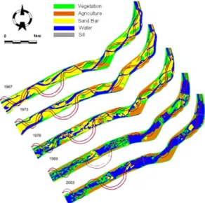
6.1. Channel Planform Geometry
From aerial photographs, three sills were visible as
early as since 1966, but the design seems to have
been completed around 1980’s. So the effect of each
sill is definitely evident after 1989. As a result, the
sand bar located just upstream of each sill has
disappeared, and vegetation has encroached just
downstream of each sill. The channel has also been
changed from sinuous to relatively straight and wide.
In terms of slope-discharge, an analysis based on Leopold and Wolman’s method results in a braided/straight channel. Lane’s method defines the channel a braided planform. The other methods of Henderson, Ackers, and Schumm and Khan showed similar results ina transition between meandering and straight planform geometry. In terms of channel morphology analysis, the Rosgen classification method indicates that this channel is an F4b at all flow conditions, but since the river has been channelized Rosgen’s classification may not be appropriate. Parker method had results from braiding/transitional to meandering/transitional planform.
In terms of stream power analysis, the Nanson and Croke method resulted in a meandering channel at low flow with braided results at high flows. Finally, the method of Chang had the same result of meandering to steep braided planform at all flow conditions.
Visual characterization of the channel was performed by channel planforms delineated using aerial photographs from 1967 to 2003 (Fig. 8). When compared with the observations from the aerial
Fig. 8. Historical Planform Change.
photographs, the methods that indicate a straight or meandering channel classification provide the best representation of the current channel characteristics.
Since the construction of sill and levee on both sides of river, the straight classification given by Leopold and Wolman’s, Henderson’s, and Schumm and Khan’s methods are the most accurate for all flow conditions. However, Mangyeong River has been channelized and is not a natural channel.
The sinuosity measured in the field was obtained from the representative 2009 survey data. This reach has relatively short distance and levee was constructed on both sides of bank along the river so the sinuosity is significantly less than 1.5. The sinuosity for the study reach was very low at 1.03.
This is definitely a straight channel and methods predicting otherwise should be questioned.
6.2. Longitudinal Profile
The thalweg elevation was calculated as the lowest point in the channel based on the surveys of MOCT (1976), IRCMA (1993), WANJUGUN (2009), and the 2009 field survey data from KICT. A thalweg comparison is conducted to determine the vertical changes in riverbed elevation at different times. The shaded area on the Fig. 9 shows the study reach area.
Overall, the study reach area has been fairly stable over the years. However, the field measurements indicate that the downstream reach has aggraded since 1976.
-10 0 10 20 30 40 50
0 10 20 30 40 50 60
Distance from Downstream (km)
Elevation (m)
1976 1993 2009
Fig. 9. Historical Thalweg Profile.
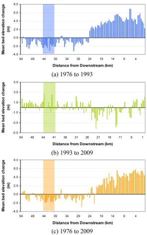
Trends in mean bed elevation were evaluated using three years in 1976, 1993, and 2009. The three comparisons can be made as 1976-1993 year, 1993- 2009 year, and 1976-2009 year. Each evaluation came from the difference between two successive survey years. This tendency shows the changes in mean bed elevation through time (Fig. 10).
-4.0 -2.0 0.0 2.0 4.0 6.0 8.0
54 49 44 39 34 29 24 19 14 9 4
Distance from Downstream (km) Mean bed elevation change (m)
(a) 1976 to 1993
-5.0 -3.0 -1.0 1.0 3.0 5.0
54 49 44 41 36 31 26 21 16 11 6 1
Distance from Downstream (km) Mean bed elevation change (m)
(b) 1993 to 2009
-4.0 -2.0 0.0 2.0 4.0 6.0 8.0
54 49 44 39 34 29 24 19 14 9 4
Distance from Downstream (km) Mean bed elevation change (m)
(c) 1976 to 2009