INTRODUCTION
The correct use of statistics in biomedical research plays an important role in enhancing the scientific quality of re- search and observing research ethics. The misuse of statis- tics is unethical and can have serious clinical consequences in medical research [1]. The misuse of statistics arises from various sources: degrees of competence of researchers in statistical theory and methods, researchers’honest errors in application of methods, egregious negligence, and deliber- ate deception [2]. Misuse of statistics means applying sta- tistical methods that are inappropriate to research goals and the data structures. The importance of careful inference was commented as part of the slow, step by step nature of scien- tific discovery [3]. A faulty understanding of statistical meth-
ods may lead, even if unintentional, to deceptive practices.
As access to user-friendly statistical packages gets easier, it is more likely that incorrect analyses are made due to mistakes by the user’s lack of fundamental statistical knowledge. These kinds of mistakes might lead to incorrect study conclusions.
In statistical analysis, the t-test is used to compare obser- vations from two populations. It tests if they have equal means or if the means of observations from two groups from one population are the same. When we deal with more than two populations or groups, we use Analysis of Variance (ANOVA) [4].
Often experimental studies measure responses two or more times repeatedly over a period on the same subject.
The use of the standard ANOVA method to compare group means is inappropriate in this kind of study, as it does not consider dependencies between observations within sub- jects in the analysis. To deal with such a context in a study, we use repeated measures ANOVA where strict analytical assumptions should be satisfied and specific analytical pro- cedures followed [5]. Failure to meet those requirements can make studies with repeated measures data vulnerable to statistical errors and can lead to incorrect conclusions [6].
In this paper, we first give examples of repeated measures
1 1
Correct Use of Repeated Measures Analysis of Variance
Eunsik Park, Ph.D.
1, Meehye Cho, B.Sc.
1, and Chang-Seok Ki, M.D.
2Department of Statistics1, College of Natural Sciences, Chonnam National University, Gwangju; Department of Laboratory Medicine and Genetics2, Samsung Medical Center, Sungkyunkwan University School of Medicine, Seoul, Korea
1 1
In biomedical research, researchers frequently use statistical procedures such as the t-test, stan- dard analysis of variance (ANOVA), or the repeated measures ANOVA to compare means between the groups of interest. There are frequently some misuses in applying these procedures since the conditions of the experiments or statistical assumptions necessary to apply these procedures are not fully taken into consideration. In this paper, we demonstrate the correct use of repeated mea- sures ANOVA to prevent or minimize ethical or scientific problems due to its misuse. We also describe the appropriate use of multiple comparison tests for follow-up analysis in repeated measures ANOVA.
Finally, we demonstrate the use of repeated measures ANOVA by using real data and the statisti- cal software package SPSS (SPSS Inc., USA). (Korean J Lab Med 2008;28:1-9)
Key Words : Ethics, ANOVA, Repeated measures, Multiple comparison
Received :December 2, 2008 Manuscript No :KJLM2206 Revision received :February 6, 2009
Accepted :February 21, 2009
Corresponding author :Eunsik Park, Ph.D.
Department of Statistics, College of Natural Sciences, Chonnam National University, 300 Yongbong-ro, Buk-gu, Gwangju 500-757, Korea
Tel : +82-62-530-3448, Fax : +82-62-530-3449 E-mail : espark02@chonnam.ac.kr
*This work was supported by a Korea Science and Engineering Foundation (KOSEF) grant funded by the Korean government (MOST) (R01-2006-000- 11087-0).
ANOVA applications in clinical chemistry and then present the correct use of repeated measures ANOVA to prevent or minimize ethical or scientific problems focusing on the experimental framework and underlining assumptions.
We also describe the use of multiple comparison proce- dures to perform follow-up analysis in repeated measures ANOVA. Then, we use real data to demonstrate the correct use of repeated measures ANOVA including follow-up pro- cedures. Finally, we conclude with a discussion.
REPEATED MEASURES ANOVA 1. Repeated measures design
Repeated measures are obtained when we measure the same variable repeatedly, for example, at different time points. Matched data can be obtained when we have sepa- rate groups but they have been matched in some way. For both cases, there is correlation among measurements within subject, or within matched pair, so standard ANOVA can- not be applied to such data.
Comparisons among treatments for matched data are per- formed by two-way ANOVA if treatments can be randomly assigned within the matched pair (a randomized block de- sign). But, for example, two-way ANOVA cannot be applied to the data of repeated measures at monthly intervals or by increasing doses where the order of time or dosage can- not be randomized. Instead, we can use repeated measures ANOVA. This design reduces variation due to differences of subjects across several treatments. Repeated-measures analysis can also handle more complex, higher-order designs with within-subject components and multifactor between- subjects components. Repeated-measures analysis can be used to assess changes over time in an outcome measured serially. Before looking at how to use repeated measures ANOVA, its examples in clinical chemistry are given below.
2. Examples in clinical chemistry
a) Cardiac troponin I was measured repeatedly over time at 2, 4, 6, and 12 hr to find out if its minor elevation was asso-
ciated with high incidence of acute myocardial infarction, cardiovascular disease, and death rate after one month [7].
This is an example of repeated measurements over time without comparison groups.
b) Twenty apparently healthy volunteers were recruited to compare the performance of two new tubes, Sekisui INSE- PACK tube and Green Cross Green Vac-Tube, with the exis- ting BD Vacutainer tubes for 49 common analytes. Results at t=24±2 hr, t=72±2 hr, and t=168±2 hr were compared with those at t=0 hr for each tube to study the stability of each analyte [8]. Since the blood sample from the same sub- ject was used for all three tubes, comparison groups of inter- est are within-subject factor. Thus, this is a study with two within-subject factors, tube types and time.
c) Blood samples were obtained before surgery and at 0, 2, 4, 6, 8, 12, 24, 48, and 72 hr after surgery to see changes in serum free or phospholipid-bound choline concentrations in response to off-pump and on-pump coronary artery bypass grafting surgery. The data represent repeated measures over time with one between-subjects group. Repeated measures ANOVA revealed a significant effect of surgery type and a significant interaction between the surgery type and time on serum free or phospholipid-bound choline concentrations, respectively [9].
Two ways may be used to analyze repeated measures for one response: the univariate approach and the multivari- ate approach [10]. The relative merits of the two approach- es, focusing on illustrating their misuses in marketing re- search, were discussed in detail [6].
In repeated measures analysis of variance, the effects of interest are a) between-subject effects (such as GROUP), b) within-subject effects (such as TIME), and c) interactions between the two types of effects (such as GROUP*TIME).
Here in parenthesis we assumed that repeated measure- ments on the same subject are taken by varying TIME and each subject belongs to one GROUP.
For tests that involve only the between-subjects effects, both the multivariate and univariate approaches give rise to the same tests. For within-subject effects and for with- in-subject-by-between-subject interaction effects, the uni- variate and multivariate approaches, however, yield differ-
ent tests. The multivariate tests provided for within-sub- jects effects and interactions involving these effects are Wilks’Lambda, Pillai’s Trace, Hotelling-Lawley Trace, and Roy’s largest root. The only assumption required for valid multivariate tests for within-subject effects is that the dependent variables in the model have a multivariate nor- mal distribution with a common covariance matrix across the between-subject effects.
The choice of a specific test statistic only becomes impor- tant when the multivariate method is applied to between- subject factors. In the case of repeated measures, all these statistics give the same F value and Pvalue. All four multi- variate tests will provide similar statistics and similar evi- dence against the null hypothesis when sample sizes are large. When samples are moderate, Pillai’s, Lawley’s, and Wilk’s have similar power [11]. Wilks’lambda is the easiest to understand and therefore the most frequently used. It has a good balance between power and assumptions. 1-Wilks’
lambda can be interpreted as the multivariate counterpart of a univariate R-squared, that is, it indicates the propor- tion of generalized variance in the dependent variables that is accounted for by the predictors. Pillai’s trace is most ro- bust with respect to violations of the assumptions of mul- tivariate ANOVA. It is particularly useful when sample sizes are small or unequal, or covariances are not homogeneous, and offers the greatest protection against Type I errors with small sample sizes. Hotelling’s trace is used when there is only one independent variable and that independent vari- able has just two conditions (i.e. two samples). Roy’s largest root is appropriate and powerful when its assumptions appear to be met and when the largest root is considerably larger compared to any of the others, but, was otherwise least sensitive. It is less robust than the other tests when the assumption of multivariate normality is violated.
The univariate tests for the within-subject effects and interactions involving these effects require some assump- tions for the probabilities provided by the ordinary F tests to be correct. Specifically, these tests require certain patterns of covariance matrices, known as Type H covariances [12]
or the sphericity assumption. Data with these patterns in the covariance matrices is said to satisfy the Huynh-Feldt
condition. When there are only two levels of the within-sub- ject effect, since a sphericity test is not needed, the usual F tests can be used to test the univariate hypotheses for the within-subject effects and associated interactions.
We need to distinguish clearly the difference between the sphericity condition and compound symmetry. Assum- ing that we have a variance-covariance matrix of the treat- ments within the group factor, we say that the data satis- fies the compound symmetry condition when all variances (on the diagonal of the covariance matrix) are equal and all covariances between treatments (off the diagonal of the covariance matrix) are equal. The compound symmetry is the sufficient condition in conducting repeated measures ANOVA but it is not the necessary one. The sphericity con- dition is a more general case of compound symmetry. It holds when the variances of the differences between the treatment levels are equal [13]. Thus, the sphericity assump- tion needs to be checked when carrying out repeated mea- sures ANOVA [15, 16].
If your data do not satisfy the sphericity condition, an adjustment to the degrees of freedom of the numerator and denominator can be used for a correction. Two such adjust- ments, based on a degrees of freedom adjustment factor, are known as ε(epsilon). Both adjustments estimate epsilon and then multiply the numerator and denominator degrees of freedom by this estimate before determining the signif- icance levels for the F tests. The first adjustment proposed by Greenhouse and Geisser is labeled Greenhouse-Geisser epsilon and represents the maximum-likelihood estimate of Box’s epsilon factor [15]. It has been shown that the estimate by Greenhouse and Geisser tends to be biased downward, that is, it is too conservative, especially for small samples [16]. Although epsilon must be in the range of 0 to 1, the estimator by Huynh and Feldt can be outside this range.
When the estimator by Huynh and Feldt is greater than 1, a value of 1 is used in all calculations for probabilities and the probabilities are not adjusted. In addition, another epsilon, the Lower-Bound epsilon, may also be used. The Lower- Bound epsilon is also referred to as part of the Greenhouse and Geisser method. The output from SPSS (SPSS Inc., Chi- cago, IL, USA) provides all three epsilons. In practice, the
first two epsilons, which are also available in SAS (SAS Institute Inc., Cary, NC, USA), are widely used to correct for the non-sphericity condition. The magnitude of the epsilons is also an indication of the violation of the spheric- ity assumption. The closer epsilon is to 1, the higher the possibility that the data satisfies the sphericity condition.
The formal method to detect the violation of the sphericity assumption is to use Mauchley’s test. It is available in widely used packages such as SPSS and SAS [14].
In summary, if your data do not meet the assumption of sphericity, use adjusted F tests. However, when you strongly suspect that your data may not have Type H covariance, all these univariate tests should be interpreted cautiously. In such cases, you should consider using multivariate tests instead.
As the assumption used in the univariate method is too re- strictive, we can use multivariate repeated measures ANOVA methods. In this case, the model is much more complicat- ed because there is no longer a nice, simple assumption about covariance. Thus, it is no longer possible to use famil- iar procedures based on simple F ratios of mean squares.
There are reasons when the univariate and multivariate tests disagree. Differences can be due to an outlier, or the requirements of one or both tests are not met by the data, or because one test has much less power than the other does where the power is the complement of the Type II error. Fur- ther study is needed to determine the cause of the disagree- ment. If univariate and multivariate analyses lead to differ- ent conclusions, it is safer trusting the multivariate statis- tic because it does not require the sphericity assumption.
However, in the case of small samples, we should consider this carefully. In this case, the reduced number of degrees of freedom for error in the multivariate approach may cause this approach to fail to identify effects that are significant in the univariate analysis. The choice between the univariate and multivariate approaches depends on some conditions of the data. The univariate approach has higher power, i.e., a smaller Type II error rate, if the sphericity assumption holds. However, many statisticians argue that this assump- tion is rarely met in practice. In this case, the use of a mul- tivariate approach is preferred, providing that the sample size is sufficiently large [15, 16].
3. Multiple comparisons
When we compare means from multiple groups of obser- vations, we first test to see if there are significant differ- ences among the means of groups. The test stops if there is no evidence of difference. Otherwise, we perform follow- up tests for multiple comparisons to determine which group mean is larger and by how much.
Two crucial statistical errors related to the mean compari- son procedures are the use of the wrong statistical tests and the inflation of the type I error [17]. The former includes some errors such as the incompatibility of the test with a specific data type such as paired or unpaired data, the incor- rect use of the parametric method, and use of an inappro- priate test for the hypothesis under investigation. Errors related to the inflation of the type I error include failures and incorrect use of multiple comparison procedures. Appro- priate multiple comparison procedure depends on the study objective and data structure.
Bonferroni’s test is a multiple comparison procedure in- volving application of the standard t-test. The significance level is adjusted by dividing it by the number of dependent comparisons to be made. This method is recommended only when there are a small number of comparisons. Otherwise, the type II error increases causing the power to become low [18]. Use of the adjusted P values was recommended for any simultaneous inference procedure, specially the Holm- Bonferroni procedure, since it is more powerful than the original Bonferroni procedure [19]. Holm’s procedure is a simple procedure that is less conservative but maintains the type I error rate, α. Here, unadjusted Pvalues are or- dered from p1to pn and then, the Pvalues are adjusted by multiplying pi with the corresponding (n-i+1). That is, the adjusted Pvalues (n-i+1)piare compared to α. In this pro- cedure, hypotheses are tested sequentially starting from the smallest Pvalue p1. The testing process stops when we receive a non-significant result. The remaining untested hypotheses are considered non-significant.
When the interaction between time and main effects exi- sts, we investigate its nature without being concerned about the main effects as these are not of practical relevance. An
interaction is the variation among the differences between the means for different levels of one factor over different time points. Thus, the common practice for multiple com- parisons in this case is to compare the mean responses of the group levels at each interval.
For multiple comparisons for the repeated measures data, the data should conform to the sphericity assumption. If this assumption is valid, we can use multiple comparison procedures for the univariate approach as in the case of standard ANOVA. We may use well-known multiple com- parison procedures or contrast tests, as they are useful to compare the means averaged over time or at individual inter- vals [18]. Little research has been conducted on the impact of a violation of the sphericity assumption on multiple com- parisons in the repeated measures ANOVA. The effect of nonsphericity was studied on the a prioritests for repeat- ed measures data [20]. It was found that even small depar- tures from sphericity can produce large biases in the F test.
If the sphericity assumption is not met, the use of the pooled error term in pair-wise comparisons can lead to a lenient or conservative Type I error rate [21]. The use of separate error terms for each comparison was recommended. The power and Type I errors was tested for five a prioritests under repeated measures conditions [22]. His main findings were that Tukey’s Wholly Significant Difference (WSD) test inflated the Type I error rate when sphericity is even slightly violated but the Bonferroni procedure was extremely robust and controlled Type I error rates. It was concluded that the Bonferroni method was the best method to use in terms of Type I errors and Tukey’s WSD was the most appropriate procedure in terms of power for a small sample. Maxwell’s work was extended for an unbalanced design [23], where the Bonferroni method was concluded to be statistically more powerful than the multivariate test especially when the number of repetitions increases.
The choice of analysis depends on complex relationships between the degree of sphericity violation and sample size [24]. If the sphericity condition of the covariance structure is satisfied, we can apply any of the multiple comparison procedures depending on the purpose of the study. Other- wise, it would be better to use Bonferroni t statistics, as
these statistics can control the type I error rate and ensure the power if the sample size is relatively large [22].
CORRECT USE OF REPEATED MEASURES ANALYSIS OF VARIANCE
In this section, we apply repeated measures ANOVA to real data. Our objective is to present the correct procedures to analyze repeatedly measured data.
1. Data structure
Twenty subjects were recruited for this study. Each subject was measured on days 0, 1, and 3 repeatedly. On each day, BD Vacutainer was compared with the two new tubes, Sek- isui INSEPACK and Green Cross Green Vac, for differences in routine hematology and coagulation test results. Thus, two within-subject factors are measured on each subject [8].
In this study, major interest lies in comparison of tube types, given as a within-subject factor. In the study of laborato- ry medicine, the major factor of interest is commonly given as a within-subject factor, while it is frequently given as a between-subject factor in other biomedical studies. We use erythrocyte sedimentation rate (mm/hr) as a response variable among routine hematology and coagulation test results to demonstrate using repeated measures ANOVA.
For repeated measures ANOVA, we need to transform the data to the multivariate form where all repeated measures of responses (Y_Dx_Ty, x=0, 1, 2 for day, y=1, 2, 3 for tube type) over day (Day) and tube type (Tube), taken from the same subject, are listed as one observation.
2. Use of SPSS
To perform the repeated measures ANOVA in Tables 3, 4 using SPSS 16.0, after creating the data set with the above
Y_D0 _T1
Y_D0 _T2
Y_D0 _T3
Y_D1 _T1
Y_D1 _T2
Y_D1 _T3
Y_D3 _T1
Y_D3 _T2
Y_D3 _T3
19 14 22 21 18 21 16 16 17
... ... ... ... ... ... ... ... ...
17 13 14 17 12 12 16 9 9
data structure, click on‘Analyze-General Linear Model- Repeated Measures’in this order on the SPSS menu window.
Next, on the pop-up window, specify within-subject fac- tor name as‘Day’and number of levels as‘3’. Repeat this for the within-subject factor‘Tube’. Then click on‘Define’
button. On the new pop-up window, move corresponding variables from the left hand list to the right side boxes for within-subjects variables and between-subject factors if you have any. Now, when the‘OK’button is clicked, then the analysis output will appear in a separate window. In front of the output window, SPSS codes are displayed before the analysis results are provided. Another way to use SPSS is to run these SPSS codes directly instead of using the menu-driven method described above.
For multiple comparisons of the repeated measures AN- OVA, click on ‘Analyze-General Linear Model-Multivari- ate’sequentially on the SPSS menu window. Next, on a pop-up window, move corresponding variables from the left hand list to the right side boxes for dependent variables and the fixed factor. Then click on the ‘Post Hoc’button to designate the post hoc multiple comparison method. On a new pop-up window, move a variable from the left hand list to the right side box for post hoc tests and check for the box next to ‘Bonferroni’to compare groups by the Bonfer- roni method. Now, if the ‘Continue’button is clicked, you can go back to the previous window where clicking on ‘OK’
button will produce output for multiple comparisons. This is useful for multiple comparisons of between-subject factors.
When there are missing values, the GLM procedure re- moves all the data for any subject that has incomplete data, while MIXED procedure still analyzes data from all the sub-
jects, even if some have missing values. Thus, use of the MIXED procedure is recommended in this case, since the presence of missing values is a less severe problem with the MIXED procedure than it can be with the GLM procedure.
3. Statistical analysis
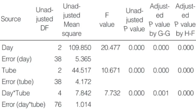
The means and standard deviations (SD) for erythrocyte sedimentation rate are given in Table 1. Mean differences between tube types vary by day; this indicates the possible existence of their interaction effect. Table 2 provides uni- variate tests for within-subject effects. The interaction effect of ‘Day’and ‘Tube’and their main effects are all signifi- cant. As their validity depends on whether or not the covari- ance structure satisfies the sphericity condition, we can use the test based on Mauchly’s Criterion to check for this condition. Pvalues for the effect ‘Day’and its interaction with ‘Tube’are 0.002 and 0.000, respectively. That is, the sphericity condition is not met, while it is 0.230 for the effect
‘Tube’. Thus, test results of the significance of ‘Day’and the interaction based on Table 2 are suspicious. The right- most two columns in Table 2 contain two adjusted Pvalues, labeled G-G and H-F. These two P values are obtained from F values with a reduced degree of freedom using Box’s method. In our example, both adjusted Pvalues from the Greenhouse-Geisser and Huynh-Feldt epsilons provide the same conclusions. This is not always the case. More com- monly, the unadjusted univariate method testing for a with- in-subject effect gives smaller Pvalues than the adjusted
Vacuum tube
Day 0
Mean SD
2
Mean SD
1
Mean SD
BD Vacutainer 8.60 7.96 9.85 9.16 7.10 6.91 Sekisui INSEPACK 7.80 7.49 8.80 8.51 6.75 6.54 Green Cross 10.70 9.19 10.40 9.16 7.40 7.16
Green-Vac-Tube
Table 1. ESR means and SDs
Abbreviation: ESR, erythrocyte sedimentation rate; SD, standard devia- tion; BD, becton dickison.
Source
Unad- justed DF
Unad- justed Mean square
F value
Unad- justed P value
Adjust- ed P value by G-G
Adjust- ed P value by H-F
Day 2 109.850 20.477 0.000 0.000 0.000
Error (day) 38 5.365
Tube 2 44.517 10.671 0.000 0.000 0.000
Error (tube) 38 4.172
Day*Tube 4 7.842 7.732 0.000 0.001 0.000
Error (day*tube) 76 1.014
Table 2. Repeated measures univariate ANOVA results
Abbreviations: ANOVA, analysis of variance; DF, degrees of freedom;
G-G, Greenhouse-Geisser Epsilon; H-F, Huynh-Feldt epsilon.
one if the sphericity condition is not satisfied.
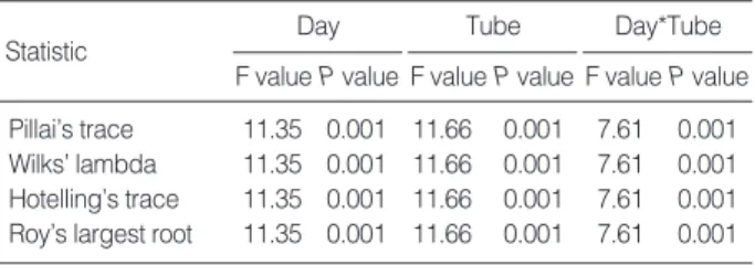
Instead of using the univariate method, we can confi- dently use the multivariate test for repeated measures data as it does not require a specific covariance structure. Table 3 shows results using the multivariate test for the signifi- cance of two within-subject effects and their interaction effect. Four statistics are given in Table 3 to accomplish the tests. Since all P values from the four statistics are 0.001, two within-subject effects and their interaction effect are significant in the models with the multivariate test.
This result agrees with that from the univariate test. There- fore, we conclude that tube types have a significantly dif- ferent effect on the response variable erythrocyte sedimen- tation rate and their effect varies by day.
4. Multiple comparisons
From previous analysis, we observe that the interaction between days and tube types is significant based on uni- variate and multivariate methods. Thus, the follow-up ana-
lysis is conducted by comparing tube types for each inter- val. Depending on the objective of the comparisons, a spe- cific multiple comparison procedure is chosen. For instance, in this illustration, our purpose is to compare two new tube types, Sekisui INSEPACK (S) and Green Cross Vac-Tube (G), with existing BD Vacutainer (B) where the number of comparisons is two. If we consider all pair-wise compar- isons, the number of comparisons to make is three. If we test for tube types at days 0, 1, and 3, the familywise prob- ability of a Type I error is 0.05 at each day, but approach- es 0.15 for the full set of comparisons. It is, therefore, desir- able to limit the number of comparisons regardless of the nature of those tests.
Since the sphericity condition is not met, the use of fol- low-up tests should be taken with care. As mentioned above in the section of multiple comparisons, the Bonferroni pro- cedure is the best one to use in terms of type I error control.
Its Pvalues were adjusted by the Holm-Bonferroni proce- dure to make it more powerful. The results are shown in Table 4. In this study, whether or not we limit the number of comparisons at each day to two or three gives the same comparison results. Note that if the interaction effect is not significant, the follow-up analysis should be carried out by comparing the tube types on response over all intervals.
For each day, we have three pairs of tube types to com- pare in the 2nd column. The 5th (4th) column of Table 4 contains the (un)adjusted Pvalues of tests while the cor- responding confidence intervals are located in the (2nd) last column. After comparing P values by the Holm-Bonfer-
Statistic Day
F value P value
Day*Tube F value P value Tube
F value P value
Pillai’s trace 11.35 0.001 11.66 0.001 7.61 0.001 Wilks’ lambda 11.35 0.001 11.66 0.001 7.61 0.001 Hotelling’s trace 11.35 0.001 11.66 0.001 7.61 0.001 Roy’s largest root 11.35 0.001 11.66 0.001 7.61 0.001 Table 3. Multivariate ANOVA tests for two within-subject effects and their interaction effect
Day Vacuum tube
comparison*
95% confidence limits using Holm-Bonferroni
procedure Unadjusted
95% confidence limits Unadjusted
P value
P value using Holm-Bonferroni
procedure Mean
difference
0 B-S 0.80 0.0608 0.0608 (-0.040, 1.640) (-0.040, 1.640)
B-G -2.10 0.0036 0.0072 (-3.423, -0.777) (-3.638, -0.562)
S-G -2.90 0.0001 0.0003 (-4.142, -1.658) (-4.458, -1.342)
1 B-S 1.05 0.0252 0.0504 (0.146, 1.954) (-0.001, 2.101)
B-G -0.55 0.2749 0.2749 (-1.574, 0.474) (-1.574, 0.474)
S-G -1.60 0.0002 0.0006 (-2.319, -0.881) (-2.501, -0.699)
3 B-S 0.35 0.3672 0.7344 (-0.443, 1.143) (-0.572, 1.272)
B-G -0.30 0.5163 0.5163 (-1.249, 0.649) (-1.249, 0.649)
S-G -0.65 0.0115 0.0345 (-1.137, -0.163) (-1.260, -0.040)
Table 4. Multiple comparisons of vacuum tube types at each day Abbreviation: ANOVA, analysis of variance.
roni procedure with the significance level 0.05, significant pairs of tube types are B-G and S-G at day 1, S-G at day 2, S-G at day 3, which vary by day due to the interaction effect between tube types and day. Since statistical signif- icance does not always imply clinical significance, clinical interpretation can differ from the statistical one.
DISCUSSION
Mean difference comparison procedures are very widely used in most biological and medical research as well as other life and social sciences. The inappropriate uses of such meth- ods may lead to wrong conclusions about the nature of dif- ferences and the relationship of factors for the outcome of interest under the comparison. Aside from the widely used procedures, such as one or two sample t-tests and some nonparametric tests, the standard ANOVA and repeated measures ANOVA have been of concern to researchers with their uses and interpretation of results, since researchers feel confused with the use of these two methods. In this paper, we classify how to choose the correct method depend- ing on the data structure and underlying statistical assump- tions. Researchers should think about their studies care- fully before they perform statistical analysis in terms of the method of measuring responses, independence among observations, and the use of appropriate models.
In our example, we demonstrated the use of repeated measures ANOVA. This example also showed how the data structure should look and how the assumption of the sphe- ricity condition is met and checked. In practice, we need to verify, before statistical analysis is carried out, whether or not responses are measured repeatedly. The sphericity as- sumption is often not satisfied. Then, we need to use some adjustment to deal with this assumption violation. We also note that this assumption is necessary for the univariate method only and its violation across repeated measures inflates a Type I error in a univariate repeated measures ANOVA. The use of the multivariate method for the repeat- ed measures ANOVA has an advantage in that it does not require the assumption on the covariance structure. In prac- tice, we may sometimes see conclusions from the two meth-
ods using univariate and multivariate analysis do not agree.
In the univariate method, if the sphericity assumption is not met, we use adjustments, such as Greenhouse-Geisser and Huynh-Feldt, to account for the within-subject correlation.
However, these adjustments may be inadequate to address the impact of the correlation and in turn may lead to a wrong conclusion. In this case, researchers should decide on which method they should rely. Our recommendation is that if the sphericity condition is met, we should use the univariate method. Otherwise, we should use the multivariate approach.
The multivariate repeated measures ANOVA has some limi- tations. Since multivariate ANOVA does not require a covari- ance structure assumption, it cannot deal with some infor- mation from the data; this in turn has an adverse impact on efficiency and power. If there is a missing observation at a single time for a given subject, the multivariate ANOVA will delete all entries of that subject; this results in loss of valid data. To avoid some of the limitations of univariate and multivariate ANOVAs, we can use a mixed model to ana- lyze the repeated measures data. We will mention this me- thod in other work as it is beyond the scope of this paper.
Another issue that needs attention when applying the repeated measure ANOVA is the use of follow-up analy- sis. Depending on the existence of an interaction effect, we should make the appropriate multiple comparisons. Choos- ing the type of multiple comparisons depends on the study objective and interpretation of interest. Some recent stud- ies show that the violation of sphericity in repeated mea- sures ANOVA has effects on the follow-up analysis in terms of the Type I error rate and power. It is safe to use the Bon- ferroni method to do the follow-up analysis as it can con- trol the type I error rate. However, to ensure the power, the Bonferroni adjustment procedure such as Holm’s method can be considered.
Finally, we mention the use of statistical packages. The most widely used statistical packages, such as SAS, SPSS, S-plus, or Stata, support standard ANOVA and repeated measures ANOVA, as well as multiple comparisons in a user-friendly way. Sometimes different software and dif- ferent methods may require preparation of different data formats to perform the same statistical analysis. Since sta-
tistical software does not check if statistical assumptions are satisfied, a prior assumption checking process is nec- essary before performing statistical analysis.
요 약
의학 연구에서t검정과 (반복측정치가 있는) 분산분석은 관심
의 대상이 되는 그룹 간 평균을 비교하는 방법으로 널리 사용되 고 있다. 이러한 통계적 방법을 올바르게 적용하기 위하여 사전 에 만족해야 할 통계적 가정을 확인하는 것은 중요하다. 본 논문 에서는 분산분석을 잘못 사용함으로 인해 발생할 수 있는 윤리적 혹은 과학적 문제를 예방하고 최소화하기 위하여, 반복측정치가 있는 분산분석의 올바른 사용법을 제시하고, 사후 분석 방법인 다중 비교법의 적절한 사용법을 함께 설명하였다. 또한 실제자료 에 SPSS (SPSS Inc., USA)를 이용한 분석과정을 제시하였다.
REFERENCES
1. Altman DG. Statistics and ethics in medical research. VIII-Improving the quality of statistics in medical journals. Br Med J 1981;282: 44-6.
2. Gardenier JS and Resnik DB. The misuse of statistics: concepts, tools, and a research agenda. Account Res 2002;9:65-74.
3. Bailar JC 3rd. Science, statistics and deception. Ann Intern Med 1986;
104:259-60.
4. Altman DG and Bland JM. Comparing several groups using analy- sis of variance. Br Med J 1996;312:1472-3.
5. Bergh DD. Problems with repeated measures analysis: Demonstra- tion with a study of the diversification and performance relation- ship. Acad Manage J 1995;38:1692-708.
6. LaTour SA and Miniard PW. The misuse of repeated measures anal- ysis in marketing research. J Mark Res 1983;20:45-57.
7. Jung CL, Cho SE, Hong KS. Clinical significance of minor elevation of Cardiac Troponin I. Korean J Lab Med 2008;28:339-45. (정채림, 조 성은, 홍기숙. Cardiac Troponin I 경도 증가의 임상적 의의. 대한진단 검사의학회지 2008;28:339-45.)
8. Oh SH and Ki CS. Comparison of two new plastic tubes (Sekisui INSEPACK and green cross green Vac-Tube) with BD Vacutainer tubes for 49 analytes. Korean J Lab Med 2007;27:69-75. (오수현및기 창석. 49종의 검사에 대한 새로운 두 종류의 플라스틱 진공채혈관(Sek- isui INSEPACK 및 녹십자 Green Vac-Tube)과 BD Vacutainer 진공 채혈관의비교. 대한진단검사의학회지 2007;27:69-75.)
9. Ilcol YO, Basagan-Mogol E, Cengiz M, Ulus IH. Elevation of serum cerebral injury markers correlates with serum choline decline after coronary artery bypass grafting surgery. Clin Chem Lab Med 2006;
44:471-8.
10. Cole JWL and Grizzle JE. Applications of multivariate analysis of variance to repeated measurements. Biometrics 1966;22:810-28.
11. Johnson RA and Wichern DW, eds. Applied multivariate statistical analysis. 6th ed. New York: Prentice Hall, 2007.
12. Huynh H and Feldt LS. Conditions under which mean square ratios in repeated measurements designs have exact F-distributions. J Am Stat Assoc 1970;65:1582-9.
13. Maxwell SE and Delaney HD, eds. Designing experiments and ana- lysing data: A model comparison perspective. Belmont: Wadsworth, 1990.
14. Atkinson G. Analysis of repeated measurements in physical thera- py research. Phys Ther Sport 2001;2:194-208.
15. Greenhouse SW and Geisser S. On methods in the analysis of pro- file data. Psychometrika 1959;24:95-112.
16. Huynh H and Feldt LS. Estimation of the box correction for degrees of freedom from sample data in the randomized block and split-plot designs. J Educ Statist 1976;1:69-82.
17. Strasak AM, Zaman Q, Pfeiffer KP, Gobel G, Ulmer H. Statistical errors in medical research-a review of common pitfalls. Swiss Med Wkly 2007;137:44-9.
18. Toothacker LE, ed. Multiple comparisons procedures: Quantitative applications in the social sciences series No. 89. Thousand Oaks:
Sage Publications, 1993.
19. Wright SP. Adjusted p-values for simultaneous inference. Biomet- rics 1992;48:1005-13.
20. Boik RJ. A priori tests in repeated measures designs: effects of non- sphericity. Psychometrika 1981;46:241-55.
21. Mitzel HC and Games PA. Circularity and multiple comparisons in repeated measures designs. Br J Math Stat Psychol 1981;34:253-9.
22. Maxwell SE. Pairwise multiple comparisons in repeated measures designs. J Educ Statist 1980;5:269-87.
23. Keselman HJ and Keselman JC. Repeated measures multiple com- parison procedures: effects of violating multisample sphericity in unbalanced designs. J Educ Statist 1988;13:215-26.
24. Atkinson G. Analysis of repeated measurements in physical thera- py research: multiple comparisons amongst level means and mul- tifactorial designs. Phys Ther Sport 2002;3:191-203.