The Relationship among Land Use, Vegetation and Surface Temperature
in Urban Areas
-The Case of Deagu City-
1)
Jae Ik KIM
1※․Chang-Hwan YEO
2도시지역 지표온도와 토지이용 및 식생상태와의 상관관계에 관한 연구
: 대구광역시의 경우
김재익
1※․여창환
2ABSTRACT
The primary purpose of this paper is to prove a clear relationship among land use type, vegetation level and surface temperature. For this purpose, this paper presents series of spatial distribution maps of the three features obtained through the visual interpretation of digital images. The result of study tells us that the spatial distribution of the vegetation level is very similar with that of surface temperature. By analyzing the relationship between surface temperature and land use types, this study categorizes the eighteen urban land uses into 7-8 groups according to their average surface temperature. The Duncan test was conducted to categorize the land uses. The surface temperature of manufacturing related land use is the highest, semi-residential use is the next, non-residential land use is the next to the lowest, and the agricultural and forest land use is the lowest. This paper provides another strong evidence of the relationship by showing the regression result.
KEYWORDS: Land Use, Surface Temperature, Vegetation Index, Land Cover, Duncan Test
요 약
본 연구는 도시지역에서 지표온도를 결정하는 요인으로서 토지이용과 식생분포를 설정하고 이
2005년 1월 12일 접수 Recieved on January 12, 2005 / 2005년 6월 20일 심사완료 Accepted on June 20, 2005 1 Associate Professor, Department of Urban Planning, College of Engineering, Keimyung University Daegu, Korea 2 Graduate Student in Ph.D Course, Department of Urban Planning, Graduate School of Engineering, Keimyung University Daegu, Korea
※ 연락저자 E-mail : [email protected]
1. BACKGROUND
There are many studies to identify the surface temperature differences in an urban area by using remote sensing data(Nicole, 1994; Jo and Lee, 2000; Kwon and Yamada, 2003). In urban areas, lands are used in various ways, such as residential, commercial, industrial, public, and so on. The difference in the land use makes the surface temperature different. Also, the surface temperature in urban areas can also be varied by vegetation levels. Therefore, it is fair to say that there exists a close relationship among land use, vegetation and surface temperature in urban areas.
The majority of urban land is covered by man-made structures, such as buildings, roads, manufacturing facilities. These structures are, of course, placed according to the land use regulations. Therefore, the land cover has deep relationship with land use. However, the term land cover and land use are distinct. Land cover refers to the physical materials on the surface of a given parcel of land(e.g. grass, concrete, tarmac, water), while land use refers to the human activity that takes place on, or makes use
of, that land(e.g. residential, commercial, industrial)(Barnsley et al, 2001,).
It is known that the structures or land cover materials make surface temperature higher in urban areas than in rural areas. There are also significant temperature differences among urban land uses mainly because different land uses make the land cover different. Many other studies also point out that the surface temperature can be determined mainly by the vegetation level. The vegetation level can also be considered as a proxy of land use because main determinant of vegetation level is land use type.
However, there is a strong tendency that researches of different origin focus only their concern. For example, natural science-oriented study focuses on vegetation conditions while social science-oriented study focuses on land use type. If the temperature on urbanized area matters for some reasons (environmental and/or health problem), then policy attention should be paid. In this case, the information on the level, change, factors and distributional characteristics of the surface temperature is essential for effective policy establishment. However, unfortunately, studies on the clear relationship 들의 상호관계를 규명하는 것을 목적으로 한다. 이를 위하여 대구광역시를 사례지역으로 위성영 상을 판독하고 그 결과를 수치지도와 중첩하여 분석을 실시하였다. 지표온도와 식생지수(표준식생 지수)는 위성영상분석을 통하여 도출하였고 토지이용자료는 통계청이 지난 2001년 제작한 기초단 위구 자료를 통하여 획득하였다.
분석결과 예상한 바와 같이 지표온도는 식생분포와 토지이용분포와 깊은 상관관계가 있는 가 운데 식생상태보다는 토지이용에 의해 더욱 많은 영향을 받는 것으로 나타났다. 이에 따라 본 연 구는 토지이용과 지표온도와의 관계규명에 초점을 두었다. 이를 위하여 본 연구는 18개로 구분된 토지이용을 표면온도에 따라 Duncan 검증방법으로 7-8개의 그룹으로 분류하였다. 이에 의하면 지표온도는 제조업과 관련된 토지이용이 많은 지역에서 가장 높았고, 그 뒤를 이어 도심상업지역 이 높았다. 반면 농업 및 임야지역의 지표온도가 가장 낮게 나타났다.
주제어: 토지이용, 표면온도, 식생지수, 토지피복, Duncan 검정
among land use, vegetation level and surface temperature are scanty. This paper is designed to show the surface temperature differences by land use type and vegetation index and to verify which factor affect more on the surface temperature.
2. STUDY AREA
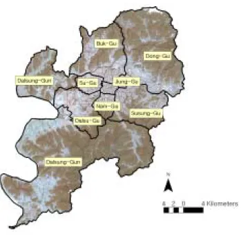
This paper employs Daegu city, the fourth largest city in Korea with population 2.8 millions in 2000 as a study area. Daegu is located in the southeastern part of Korea. Geographical feature of Daegu city can be summarized as a basin - a flat plain surrounded by mountains. Figure 1 shows the boundaries of the study area that includes eight local government boundaries.
Daegu area is selected as study area because researchers have information and knowledge about the city in depth and thus easy to check and confirm any uncertain data and information.
3. DATA AND APPROACH
This paper utilizes Landsat TM 5 imagery of 2000(October 16) of Daegu city to derive vegetation index and to measure average surface temperature. The land use data was not available in primary administration unit until 2000. Even worse, the existing land use maps need more detailed ground survey. Under these circumstances, digital images acquired by satellite sensors can be a reasonable substitute for conventional land use maps. Fortunately, however, Korea National Statistical Office established “the basic survey unit” which is similar with the census block in year 2001, and thus, the land use data is available by the basic survey unit. It provides 18 land use types along with primary information on population and housing(see Table 1 and Figure 4 for the land use classification and spatial distribution by land use).
FIGURE 1. Study area
The satellite data were examined using standard image processing software, ERDAS (v.8.6) and ERDAS IMAGINE, and the results of the digital processing were presented with ARCVIEW(v.3.3). The statistical analyses were performed by using SAS package. The satellite image was transformed into Transverse Mercator(TM) coordinate system by using 1/25000-scale standard topographic maps.
Geometric correction was based on the first order polynomial equations. The pixel size was maintained at 30m.
4. SURFACE TEMPERATURE, VEGETATION AND LAND
USE TYPES
4-1 Surface temperature distribution
The surface temperature was calculated by the following conversion formula.
T = K2 ln ( K1
L
λ+1) where
T: effective at-satellite temperature in kelvin;
K2: calibration constant 2 in kelvin;
K1: calibration constant 1 in W/(㎡․sr․㎛ );
L: spectral radiance at the sensor‘s aperture;
and
L
λ= ( LMAX
λ- LMIN
λQ
cal max) Q
cal max+LMIN
λwhere
L
λ: spectral radiance at the sensor‘s aperture in W/(㎡․sr․㎛);
Q
cal: quantized calibrated pixel value in DNs;
Q
cal min: minimum quantized calibrated pixel value (DN ) corresponding to LMIN
λQ
cal max: maximum quantized calibrated pixel value (DN) corresponding to LMAX
λLMIN
λ: spectral radiance that is scaled to Q
cal minin W/(㎡․sr․㎛);
LMAX
λ: spectral radiance that is scaled to Q
cal maxin W/(㎡․sr․㎛).
Authors recommend to read Chander and Markham(2003) for more information on these formula and related calculations.
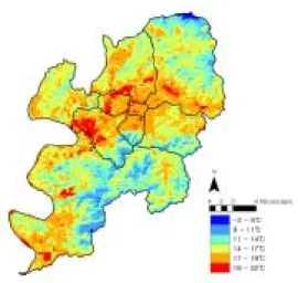
Figure 2 illustrates the surface temperature distribution of the study area. The figure tells us that the surface temperature of urbanized areas with over 17℃ is higher than that of non-urban areas with below 14℃ in general. The surface temperature is the lowest in mountainous areas and the highest in urban centers and traditional manufacturing areas. In addition, high temperature areas are observed along east-west axis of the city.
FIGURE 2. The Surface Temperature: Daegu City
4-2. Spatial distribution of vegetation index
Vegetation level refers the density of green vegetation across the Earth's landscapes. It can be measured by using satellite sensors that observe the distinct wavelengths of visible and near-infrared sunlight that is absorbed and reflected by the plants. The vegetation index(VI) ranges from 0 to 255(0=a pure black pixel, 255=a pure white pixel, and all the numbers between=gray). By subtracting the red light images from the near-infrared image, everything that has about the same brightness level in the two wavelengths becomes dark, and everything that is brighter in the near-infrared becomes light. The VI range of study area begins from 15 and up to 255. The low value of VI in certain area implies that the area is close to the natural condition. One shortcomings of the VI in this study is that the VI of water is considered the lowest vegetation index with 15-100 which is almost the same as urbanized area. But this cannot ruin the confidence of analysis results, because the portion is small.
The vegetation level is frequently converted into NDVI(Normalized Difference Vegetation Index) range from -1 to +1 by calculating the following equation.
NDVI = Band4 - Band3 Band4 + Band3
where "Band4" is near-infrared light, and
"Band3" is red light. NDVI can be interpreted as the difference in reflectance is divided by the sum of the two reflectances. An NDVI value of -1 means no green vegetation and close to +1 (usually 0.8-0.9) indicates the highest possible
density of green leaves. This study utilizes the NDVI since it is most commonly used index for satellite imagery.
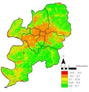
By comparing Figure 3 with Figure 2, it is easy to find out that the spatial distribution of the vegetation level is very similar with that of surface temperature.
FIGURE 3. NDVI: Daegu City 4-3. Spatial distribution of land use
Figure 4 shows the land use distribution map
constructed based on the basic survey unit
information. Land Use Classification by the Basic
Survey Unit is presented in Table 1. As shown in
Figure 4, the urbanized areas(residential,
semi-residential, and non-residential use) are
surrounded by rural uses. In the case of
urbanized areas, non-residential use, especially
commercial use, is surrounded by the residential
use in general. The manufacturing activity is
located northwestern part of the city and outer
southwestern edge of the urbanized area.
FIGURE 4. The land use distribution: Daegu City 4-4. The relationship among land use
types, vegetation and surface temperature
The surface temperature and vegetation index
are quantitative variables. Their relationship can easily be measured by many ways. But the land use number is not a variable. Therefore, one can compare the surface temperature with vegetation index quantitatively, but cannot compare the surface temperature with land use directly. By combining the three figures, however, the difference of the surface temperature by land use type and by vegetation index can be derived clearly.
First of all, by combining surface temperature information with land use information, the highest temperature is found at manufacturing and commercial areas, with surface temperature higher than 19℃.
Before test the strong relationships between land uses and surface temperature, this study checks if there exists surface temperature differences by land use type. The ANOVA test
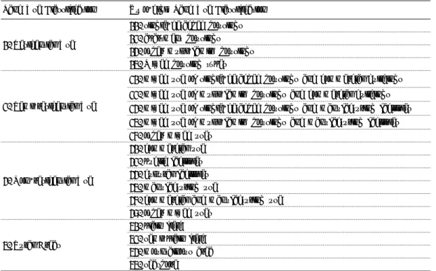
TABLE 1. Land use classification by the basic survey unit
Land Use Classification Two-digit Land Use Classification1. Residential Use
11. single-detached housings 12. apartment housings 13. other multi-family housings 14. Mixed housing types
2. Semi-residential Use
21. mixed use of single-detached housings and commercial buildings 22. mixed use of multi-family housings and commercial buildings 23. mixed use of single-detached housings and manufacturing facilities 24. mixed use of multi-family housings and manufacturing facilities 25. other mixed uses
3. Non-residential Use
31. commercial use 32. public facilities 33. cultural facilities 34. manufacturing use
35. commercial and manufacturing use 36. other mixed uses
4. Rural Areas
41. plain field 42. semi-plain field 43. mountainous area 44. seashore
statistics provide clear evidence of surface temperature differences by land use type with F-value 654.84 and Pr<0.0001.
One step further, the eighteen land use types are grouped based on results of Duncan method, or similarity of the average surface temperatures.
Table 2 shows the Duncan grouping by land use type. In Duncan method, means with the same letter are not significantly different.
According to the table, the highest surface temperature is found at manufacturing use with average temperature 20.8℃. The next highest group consists of mixed use of commercial and manufacturing use, mixed use of single-detached housings and manufacturing, and mixed use of multi-family housings and manufacturing – all land uses are related with manufacturing use.
This result implies that there is a strong relationship between land use types and surface
temperature.
A special attention should be given to the surface temperature of apartment housings, the major housing types of new housing construction. It is extremely low - even lower than the temperature of the single family housing areas. This difference may stem from building material difference-especially roofing materials.
Most of apartment structures are covered with concrete and apartment sites have planned open space required by the law. By contrast, the roofing material of most single-family house is a tile and there is no regal requirement for open space for the single-family housing areas.
In addition, the correlation coefficient between surface temperature and vegetation index is - 0.34 at Pr<0.0001. This a clear evidence of close relationship between surface temperature and vegetation index, though not as TABLE 2. Duncan grouping by land use type
Duncan
Grouping Mean N Land Use
A 20.81 482 manufacturing use(34)
B 19.20 72 commercial and manufacturing use(35) B 19.11 160 single-detached housings + manufacturing(23) B 19.01 4 multi-family housings + manufacturing(24)
C 18.27 653 commercial use(31)
C 18.18 2,130 single-detached housings + commercial use(21) C 18.17 696 other semi-residential mixed uses(25)
D C 18.04 5,280 single-detached housing (11)
D C 18.04 71 multi-family housings + commercial use(22)
D C 17.93 733 mixed housing types(14)
D E 17.64 421 public facilities(32)
D E 17.56 113 other multi-family housings(13) D E 17.54 163 other non-residential mixed uses(36)
F E 17.18 12 cultural facilities(33)
F 17.06 78 plain field(41)
F G 16.83 4,022 apartment housings(12)
G 16.42 302 semi-plain field(42) H 14.55 298 mountainous area(43)
strong as expected.
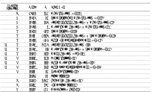
These findings can be further verified by regression analysis. By regressing vegetation index and land use types on surface temperature, this study obtains strong statistical evidence of the relationships among the three variables as shown in Table 3. The effect of land use is measured by using dummy variables. The method of avoiding dummy variable trap is a delete one category method, which measures deviation from deleted variable(mean value of single housing residential area, 18.04℃). In Table 3, the negative relationship between
surface temperature and vegetation index is derived as expected. Among dummy variables, negative(positive) values represent lower(higher) temperature than average value of the deleted variable.
5. CONCLUSION
This paper presents series of spatial distribution maps of surface temperature, vegetation and land use through the visual interpretation of multi-spectral images. There is a clear relationship among surface temperature, TABLE 3. The regression analysis
Variables Parameter
Estimate Standard
Error t -Value Pr > |t|
Intercept 20.2837*** 0.0817 248.3900 <.0001
VI: vegetation index -0.0186*** 0.0007 -27.9600 <.0001
D2: apartment housings(12) -1.1616*** 0.0222 -52.2400 <.0001
D3: other multi-family housings(13) -0.2808*** 0.1010 -2.7800 0.0055 D4: Mixed housing types(14) -0.0699 * 0.0418 -1.6700 0.0944 D5: mixed use of single-detached housings and
commercial buildings(21) 0.1294*** 0.0272 4.7500 <.0001
D6: mixed use of multi-family housings and
commercial buildings(22) -0.0138 0.1266 -0.1100 0.9134
D7: mixed use of single-detached housings and
manufacturing facilities(23) 1.1853*** 0.0852 13.9200 <.0001
D8: mixed use of multi-family housings and
manufacturing facilities(24) 1.0676 ** 0.5302 2.0100 0.0441
D9: other mixed uses(25) 0.2396*** 0.0429 5.5800 <.0001
D10: commercial use(31) 0.1825*** 0.0440 4.1500 <.0001
D11: public facilities(32) -0.2154*** 0.0541 -3.9800 <.0001
D12: cultural facilities(33) -0.3716 0.3068 -1.2100 0.2259
D13: manufacturing use(34) 2.8765*** 0.0506 56.8700 <.0001
D14: commercial and manufacturing use(35) 1.2283*** 0.1258 9.7600 <.0001
D15: other mixed uses(36) -0.2851*** 0.0846 -3.3700 0.0008
D16: plain field(41) -0.2348 * 0.1238 -1.9000 0.0579
D17: semi-plain field(42) -0.7591*** 0.0698 -10.8800 <.0001
D18: mountainous area(43) -2.1754*** 0.0786 -27.6900 <.0001
R2= 0.4431, Adj R2= 0.4425 n=15,690
***, **, * : significant at (=0.01, 0.05 and 0.10 respectively.