논문 2011-48SP-3-3
그래디언트와 상관관계의 국부통계를 이용한 얼굴 인식
( Face Recognition Using Local Statistics of Gradients and Correlations )
구 영 애*, 소 현 주**, 김 남 철****
( Yingai Ju, Hyun Joo So, and Nam Chul Kim )
요 약
지금까지 많은 얼굴 인식 방법들이 제안되었으나, 대부분의 방법들은 특징추출 과정 없이 입력 영상을 1차원 형태의 벡터로 변형한 것을 1차원 특징 벡터로 사용하거나 또는 입력 영상 자체를 특징 매트릭스로 사용하였다. 이와같이 영상 자체를 특징 으로 사용하면 조명변화가 심한 데이터베이스에서는 성능이 좋지 않는 것으로 알려져 있다. 본 논문에서는 조명변화에 효과적 인 그래디언트와 상관관계의 국부통계를 이용하여 얼굴을 인식하는 방법을 제안하였다. BDIP(block difference of inverse probabilities)는 그래디언트의 국부 통계이다. 그리고 BVLC(block variation of local correlation coefficients)의 두 타입은 상관 관계의 국부 통계이다. 입력영상이 얼굴인식 시스템에 들어 오면 먼저 BDIP, BVLC1, BVLC2의 특징 영상을 추출하고 융합한 후, (2D)2 PCA 변환을 거쳐 특징 매트릭스를 얻어서 훈련특징 매트릭스와의 거리를 구하여 최근린 분류기를 이용하여 얼굴 영상을 인식한다. 네 가지 얼굴 데이터베이스, FERET, Weizmann, Yale B, Yale에 대한 실험결과로부터, 제안한 방법이 실험 한 여섯 가지 방법 중에서 조명과 얼굴 표정의 변화에 가장 견실하다는 것을 알 수 있었다.
Abstract
Until now, many face recognition methods have been proposed, most of them use a 1-dimensional feature vector which is vectorized the input image without feature extraction process or input image itself is used as a feature matrix. It is known that the face recognition methods using raw image yield deteriorated performance in databases whose have severe illumination changes. In this paper, we propose a face recognition method using local statistics of gradients and correlations which are good for illumination changes. BDIP (block difference of inverse probabilities) is chosen as a local statistics of gradients and two types of BVLC (block variation of local correlation coefficients) is chosen as local statistics of correlations. When a input image enters the system, it extracts the BDIP, BVLC1 and BVLC2 feature images, fuses them, obtaining feature matrix by (2D)2 PCA transformation, and classifies it with training feature matrix by nearest classifier. From experiment results of four face databases, FERET, Weizmann, Yale B, Yale, we can see that the proposed method is more reliable than other six methods in lighting and facial expression.
Keywords : face recognition, local gradient, local correlation, (2D)2 PCA
Ⅰ. INTRODUCTION
Over the past few decades, face recognition has received significant attention because of its wide applications in entertainment, information security, law enforcement, and surveillance, and so on[1~2]. One
* 학생회원, ** 정회원, *** 정회원-교신저자, 경북대학교
IT대학 전자공학부
(School of Electronics Engineering, College of IT Engineering, Kyungpook National University) 접수일자: 2010년9월8일, 수정완료일: 2011년2월14일
of the most simple and well-known methods is eigenface technology[3], which is based on principal component analysis (PCA), also known as Karhunen Loeve expansion. It includes a linear core process that projects the high-dimensional data onto a lower dimensional space, based on second-order dependencies. Bartlett et al.[4] further indicated that important information on face recognition may be contained in high-order relationships among facial pixels and hence presented two different independent
component analysis (ICA) architectures, which are shown to outperform PCA. However, Yang et al.[5]
claimed that the two ICA architectures involve PCA process, whitening process, and pure ICA projection, and showed that pure ICA projection has only a little effect on the performance of face recognition.
In face recognition using PCA or whitened PCA, two-dimensional images should be converted into one-dimensional vectors at the first stage. However, as a significant extension of traditional PCA, Yang et al. proposed two-dimensional PCA (2D PCA)[6~7], also named as image principle component analysis (IMPCA), which does not need to convert an image into a vector first. Although the performance of face recognition using 2D PCA is known to be higher than that using PCA, it has been shown that it needs many more coefficients for face recognition than PCA. Therefore Zhang et al. proposed two-directional two-dimensional PCA ((2D)2 PCA)[8], which needs more less coefficients for face recognition but the recognition accuracy is the same or higher in most cases. One of the most important factors to degrade the performance of face recognition is known to be the illumination variation problem. Many methods have been proposed to solve this problem. They can be divided into three groups. The first one preprocesses an image by using an image processing technique to normalize the image. For example, logarithm transformation[9] and histogram equalization (HE)[10] are often used for illumination normalization.
However, it is difficult to deal with different lighting conditions. Recently, block-based histogram equalization (BHE)[11] has been proposed to handle the illumination variation problem, whose recognition rates are a little higher than those of HE but still not satisfactory.
The second one constructs a 3D face model for rendering-or-synthesizing face images in different illuminations and poses[12]. Its main idea is that face images with different illumination can be represented by using an illumination convex cone, which can be approximated by low-dimensional linear subspace.
But the 3D face model-based method needs many training samples with different illuminations, which is not practical.
The third effective one tries to extract illumination invariant features based on Lambertian model. For instance, self-quotient image (SQI)[13], logarithmic total variation (LTV)[14], gradientface[15], and so on.
SQI is obtained by dividing an image by its smoothed version. Although this method is simple, the use of a weighted Gaussian filter has difficulty in keeping sharp edges in low frequency illumination fields. The LTV method overcomes the shortcomings of SQI but has quite high computational expense.
The gradientface method transforms an image into its gradientface, which is known to be more insensitive to illumination than the above methods.
Related to the third method, which tries to extract illumination invariant features, it is also worthy of notice that BDIP (block difference of inverse probabilities) and BVLC (block variation of local correlation coefficients) operators, which have been applied to image retrieval[16~17], face detection[18], ROI determination[19], and texture classification[20], and yielded very good results. Both of the operators are bounded and well locally normalized to be robust to illumination variation. BDIP is a kind of nonlinear operator normalized by local maximum, which is known to effectively measure local bright variations.
BVLC is a maximal difference between local correlations according to orientations normalized by local variance, which is known to measure texture smoothness well[20].
In this paper, we apply the two operators to extracting three types of facial features. The fusion of the three features is transformed by (2D)2 PCA and classified by the nearest neighbor classifier. The results show that the proposed method using the fusion of the features is more robust to variations of illumination and expression.
The rest of this thesis is organized as follows.
Section Ⅱ will give a simple description of face recognition using PCA, whitened PCA, and (2D)2
PCA and explain some typical features. The proposed method is described in section Ⅲ and the experimental results in section Ⅳ. Finally, the conclusion is shown in section Ⅴ.
Ⅱ. TYPICAL FACE RECOGNITION METHODS AND THEIR FEATURES
In this section, we will describe typical face recognition methods using PCA and some PCA extensions, such as whitened PCA (WPCA) and (2D)2 PCA, and explain some features applied in face recognition and image retrieval areas.
2.1. Overview of face recognition using PCA or whitened PCA
Fig. 1 shows the block diagram of a typical face recognition using PCA or WPCA. In the training phase, the feature vectors are first formed from training images in a database (DB) and their mean vector, eigenvectors, and eigenvalues are computed.
The training feature vectors are next horizontally centered and finally transformed by PCA or WPCA to get transformed feature vectors. In the testing phase, a test feature vector is extracted from a test image, horizontally centered, transformed by PCA or WPCA, and compared with the transformed training feature vectors to obtain a classification result.
Suppose that there are
L
training images I1, I2, …, IL. These are then converted into one-dimensional vectors v1, v2, …, vL in the feature formation stage.The mean vector and covariance matrix are written as
μ
} { }, {ψi li
그림 1. PCA나 whitened PCA를 사용한 기존의 얼굴인 식 방법의 블록도
Fig. 1. Block diagram of a typical face recognition using PCA or whitened PCA.
μ
v
(1)
and S
X XT
(2)
where X = [x1, x2, …, xL] stands for matrix consisting of horizontally centered vectors xi = vi
- μ
fori
= 1, 2, …,L
.It should be noted here that since facial feature vectors often have tremendous dimensions, it is not tractable to directly find the eigenvectors and eigenvalues of the covariance matrix given in (2).
Instead, we can find them from the matrix G
XTX
(3)
That is, the set of
L
largest eigenvaluesλ
1 ≥λ
2 ≥… ≥
λ
L of S is identical to the set ofL
eigenvalues of G and their eigenvectors ψ1, ψ2, …, ψL of S are given as[3]ψ ∥X β∥
X β
(4)
where βi denotes the eigenvector of G corresponding to λi for
i
= 1, 2, …,L
. Selectingl
meaningful eigenvalues wherel
<L
[3], then the PCA transformed vector yi is computed byy ψ ψ ⋯ ψx
(5)
The WPCA transformed vector yi is then computed byy
ψ
ψ
⋯
ψ
x(6)
fori
= 1, 2, …,L
.In the testing phase, for the vector vts formed from a test image Its, the transformed vector yts is calculated by
y ψ ψ ⋯ ψx
(7)
with xts = vts
- μ
in PCA ory
ψ
ψ ⋯
ψ
x(8)
in WPCA.The cosine distance between the test vector and the ith transformed training vector is then computed by using
∥y∥∥y∥
y⋅y
i = 1, 2, …, L. (9)
Finally, the test image is classified to the class of ther
th training image which gives the maximum distance as ∈ ⋯ arg max
(10)
2.2 Overview of face recognition using (2D)
2PCA
The main idea of (2D)2 PCA is to perform 2-D separable KL transformation on
M
×N
images Ii, which yieldsq
×d
feature matrices[8] as follows:P ΦIΦ
,
i= 1, 2, …,
L. (11)
where ΦH and ΦV are the eigenvector matrix corresponding to thed
largest eigenvalues of the horizontal covariance matrix CH and that to theq
largest eigenvalues of the vertical covariance matrix CV, respectively. The matrices CH and CV are defined asC
I I I I
(12)
andC
I I I I (13)
where I and I denote the
m
th row vector andn
th column vector of image Ii, respectively. The vectors I and I
denote the
m
th row vector and nth column vector of the mean of the all training images Ii, respectively. The mean images I isdefined as
I
I
. (14)
Supposing there is a test image Its, we can obtain its feature matrix by
P ΓIΩ
(15)
Then the distance between the test feature matrix and the
i
th training matrix is computed by
∥
P P ∥
, i = 1, 2, …, L (16)
where P(k) denotes the
k
th column vector of a feature matrix, and ||․||2 denotes the Euclidian distance between the two feature matrices.Finally, the test image is classified to the class of the
r
th training image which gives the minimum distance as ∈ ⋯ arg min
. (17)
If we consider a horizontal projection only, it becomes a horizontal 2D PCA[6~7], whose feature matrix of size
M
×d
is given asP IΦ
, i = 1, 2, …, L (18)
and if we deal with a vertical projection only, it becomes a vertical 2D PCA[6~7], whose feature matrix of sizeq
×N
is given asP ΦI
, i = 1, 2, …, L. (19)
2.3. Typical features
Up to now various face recognition methods have been suggested, most of which without feature extraction use the one-dimensional vector stacked from a raw image or a raw image itself for a feature vector or matrix. However, a raw image is seemed to be susceptible to variation of illumination and facial expression. In this section, we thus introduce more robust features useful for face recognition.
2.3.1 Gradientface
A gradientface of an image I is defined as[16]
tan
∇ ∇
(20)
where
I
p denotes the intensity at a pixelp
of an image I. The gradients ∇
and ∇
are the derivatives of a 2-D Gaussian kernel function with varianceσ
2 in the horizontal and vertical direction, respectively.2.3.2 BDIP
BDIP for an image I is defined as
(21)
where <
․
>R denotes the averaged value over the pixelsq
’s in a moving windowR
, and
and
stand for the maximum value and mean value over the window whose center is atp
, respectively. Since the quantity within <․
>R means the gradient of a pixel,D
p implies the mean of normalized gradients over the local region whose center is atp
. As it is normalized by the local maximum, it is expected to be robust to variation of illumination. For stabilization, the denominator in Eq. (21) is clipped as max
with a thresholdδ
D.2.3.3 BVLC
BVLC for an image I is defined as
∈
max
∈
min
(22)
where
ρ
p(d
) is the local correlation coefficient along a directiond
at a pixelp
. It is defined as
, d ∈ O (23)
where
andVar
(I
p) stand for the mean and variance over the windowR
whose center is atp
, respectively,
andVar
(I
p+d) the mean andvariance of the moving window
R
whose center is at the pixelp
+d
, respectively.O
denotes a set of orientations, which may be chosen asO
= {(-k
, 0), (k
, 0), (0, -k
), (0,k
)}. Sinceρ
p(d
) means the correlation coefficient along a directiond
,C
p in Eq.(22) implies the maximum deviation of correlation coefficients over the local region whose center is at
p
. As it normalized by local standard deviations, it is also expected to be robust to variation of illumination.For stabilization, the variances in the denominator of Eq. (23) are clipped with a threshold
δ
V.Ⅲ. PROPOSED METHOD
In this section, we will describe our face recognition method whose block diagram is shown in Fig. 2. When a test image Its enters the system, it first extracts three types of features and fuses the three into a feature image I. Next, it obtains a test feature matrix transformed by (2D)2 PCA process.
The system finally classifies the test feature matrix by comparing it with the training feature matrices in a DB.
One of the three types of features used in the proposed method is the BDIP defined in Eq. (21) and the others are the two types of the BVLC. In order to distinguish them from each other, we redefine the BVLC in terms of the distance
k
as follows:
∈
max
∈
min
(24)
where
O
k denotes a set of four orientations according tok
. For simplicity, we call them BVLC1 and BVLC2 in case ofk
= 1 andk
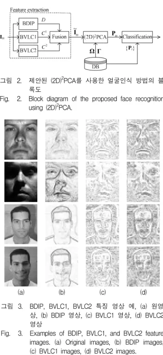
= 2, respectively.Examples of BDIP, BVLC1, and BVLC2 feature images are illustrated in Fig. 3. The first column (a) consists of four original images taken from Yale B and Weizmann DB. The former is chosen for lighting variant experiment and the latter for lighting plus expression variant experiments. The first two original images come from Subset 1 and Subset 4 of Yale B DB and the last two from the training set, and Subset 3 of Weizmann.
Γ C1
C2
Its
~
Pts
Ω
그림 2. 제안된 (2D)2PCA를 사용한 얼굴인식 방법의 블 록도
Fig. 2. Block diagram of the proposed face recognition using (2D)2PCA.
(a) (b) (c) (d)
그림 3. BDIP, BVLC1, BVLC2 특징 영상 예, (a) 원영 상, (b) BDIP 영상, (c) BVLC1 영상, (d) BVLC2 영상
Fig. 3. Examples of BDIP, BVLC1, and BVLC2 feature images. (a) Original images, (b) BDIP images, (c) BVLC1 images, (d) BVLC2 images.
The first two original images come from Subset 1 and Subset 4 of Yale B DB and the last two from the training set, and Subset 3 of Weizmann. The second column (b) corresponds to the BDIP images, the third (c) to the BVLC1 images, the fourth (d) to the BVLC2 images.
We can see from Fig. 3 that BDIP, BVLC1, and BVLC2 images are shown to be features different from raw images. It is shown that BDIP can extract sketch-like feature images, where edges and valleys around the eyes and lips are more emphasized both
for the normal image and the shadowy image. We also see that BVLC1 and BVLC2 can extract features around eyes, noses, and lips region well. Since the texture features BDIP, BVLC1 and BVLC2 are normalized well, all of them seem helpful to overcome variation of illumination. In addition, even though facial expressions change, the property of facial textures does not change so much, so that all of them look less sensitive to variation of facial expression.
Extracting BDIP, BVLC1, and BVLC2 images from a test image, the system forms the test feature image
I by fusing the three feature images. That is
I
= [ D , C
1, C
2] (25)
whereD
,C
1, andC
2 denote BDIP , BVLC1, and BVLC2 images, respectively. AnM
×N
test image yields anM
× 3N
feature image.Then we can obtain its feature matrix by using Eq. (15), calculate the distance between the test feature matrix and each of training feature matrices by Eq. (16) and finally classify it by Eq. (17).
Ⅳ. EXPERIMENT RESULTS
In this section, the performance of the proposed approach is evaluated with four face DBs: FERET[21], Weizmann[22], Yale B[22], and Yale[23]. The facial parts of images in FERET, Yale B, and Yale are cropped and resized to images of pixels without rotation and those in Weizmann are resized to images of 112×92 pixels without cropping.
For performance comparison, we implement not only our method but also other methods using raw image, gradientface, BDIP, BVLC1, and BVLC2, respectively. As for gradientface, the parameter σ of the Gaussian kernel is set to 0.1. As for BDIP and BVLCs, the clipping thresholds are set to
δ
D = 2 and toδ
V = 0.001, respectively. The performance of face recognition is measured as the averaged recognition rate, which is defined as the ratio of the number of test images classified correctly to the number of allthe test images.
4.1 Results on FERET DB
For FERET, we select 1196 images for 1196
(a)
(b)
(c)
(d)
그림 4. FERET DB의 시험 영상 집합 FB에서 선택된 고유치 개수에 따른 인식율
(a) PCA, (b) WPCA, (c) 2D PCA, (d) (2D)2 PCA Fig. 4. Recognition rates according to the number of selected eigenvalues for the probe set FB in FERET DB: (a) PCA, (b) WPCA, (c) 2D PCA, (d) (2D)2 PCA.
persons in the gallery set for training, 1195 images in the probe set FB for expression variant test, and 194 images in the probe set FC for lighting variant
(a)
(b)
(c)
(d)
그림 5. FERET DB의 시험 영상 집합 FC에서 선택된 고유치 개수에 따른 인식율,
(a) PCA, (b) WPCA, (c) 2D PCA, (d) (2D)2 PCA Fig. 5. Recognition rates according to the number of selected eigenvalues for the probe set FC in FERET DB: (a) PCA, (b) WPCA, (c) 2D PCA, (d) (2D)2 PCA.
Analysis
schemes PCA WPCA 2D PCA (2D)2PCA
Test Feature
Expression Variant
Lighting Variant
Expression Variant
Lighting Variant
Expression Variant
Lighting Variant
Expression Variant
Lighting Variant
Raw 70.96 3.61 67.11 61.34 73.97 5.15 71.63 6.19
gradientface 68.28 30.93 72.89 44.85 75.40 52.58 75.82 48.45
BDIP 61.84 60.82 59.25 54.64 66.28 57.22 63.77 56.19
BVLC1 76.23 53.09 74.06 55.15 75.40 57.73 77.41 64.95
BVLC2 76.74 59.79 82.26 62.37 75.48 65.46 76.82 57.73
Proposed 80.25 72.68 83.60 73.71 80.50 76.80 80.84 77.32
표 1. FERET DB에 대한 다양한 얼굴인식 방법의 분석 방법에 따른 최고 인식율[%]
Table 1. The highest recognition rates [%] of six face recognition methods according to various analysis schemes for FERET DB.
Analysis
schemes PCA WPCA 2D PCA (2D)2PCA
Test Feature
Expression plus lighting
Expression plus lighting
Expression plus lighting
Expression plus lighting Raw 57.5 (126) 85.19 (125) 99.62 (112x3) 99.62 (5x5) gradientface 96.35 (123) 98.65 (127) 99.62 (112x18) 97.69
(20x20) BDIP 92.69 (129) 92.12 (65) 99.23 (112x5) 99.62 (9x9) BVLC1 98.85 (118) 98.65 (114) 100 (112x5) 99.23 (6x6) BVLC2 99.04 (121) 98.46 (91) 100 (112x7) 99.23
(13x13) Proposed 99.23 (90) 99.23 (121) 100 (112x7) 100 (9x9) 표 2. Weizmann DB에 대한 다양한 얼굴인식 방법의 분석 방법에 따른 최고 인식율[%]
Table 2. The highest recognition rates [%] of six face recognition methods according to various analysis schemes for Weizmann DB.
test. Fig. 4 and Fig. 5 show the recognition rates of six face recognition methods according to the number of selected eigenvalues for the probe set FB and for the probe set FC, respectively. Table 1 lists their highest recognition rates.
From Table 1, we can see that the performance of the gradientface feature is not higher than that of the raw image feature in expression variant test over PCA, and much lower than that of the raw image feature in lighting variant test over WPCA. However, the performance of the fusion of BDIP and BVLCs features is higher than that of the raw image feature and that of the gradientface feature over PCA, WPCA, 2D PCA, and (2D)2 PCA. It achieves the best result for expression variant test over WPCA and for lighting variant test over (2D)2 PCA. It also gives the gain of maximum 71.13% over the raw image feature
and that of 41.75% over the gradientface feature.
4.2 Results on Weizmann DB
For Weizmann, we select 130 images for 26 persons in the training set for training, and 520 images in Subset 3 for expression plus lighting variant test. The highest recognition rates and the numbers of selected eigenvalues are listed in Table 2.
From Table 2, we can see that the performance of the gradientface feature is not higher than that of the raw image feature in expression plus lighting variant test over (2D)2 PCA. However, the performance of the fusion of BDIP and BVLCs features is higher than that of the raw image feature and that of the gradientface feature, and achieves 100% over 2D PCA and (2D)2 PCA.
Analysis
schemes PCA WPCA 2D PCA (2D)2PCA
Test Feature
Lighting Variant
Lighting Variant
Lighting Variant
Lighting Variant
Raw 39.29 (38) 88.57 (36) 47.86 (112x19) 46.43
(20x20) gradientface 93.57 (80) 98.57 (59) 94.29 (112x20) 92.14
(20x20)
BDIP 92.86 (11) 98.57 (12) 99.29 (112x10) 99.29
(16x16)
BVLC1 97.86 (15) 97.86 (11) 96.43 (112x19) 99.29
(12x12)
BVLC2 97.14 (10) 97.86 (11) 94.29 (112x13) 99.29
(14x14) Proposed 99.29 (11) 99.29 (10) 99.29 (112x12) 99.29
(17x17) 표 3. Yale B DB에 대한 다양한 얼굴인식 방법의 분석 방법에 따른 최고 인식율[%]
Table 3. The highest recognition rates [%] of six face recognition methods according to various analysis schemes for Yale B DB.
Analysis
schemes PCA WPCA 2D PCA (2D)2PCA
Test Feature
Expression Variant
Expression Variant
Expression Variant
Expression Variant Raw 98.67 (9) 100 (10) 100 (112x6) 100 (5x5) gradientface 89.33 (14) 90.67 (12) 93.33 (112x19) 92.00 (9x9) BDIP 98.67 (9) 98.67 (9) 100 (112x4) 100 (4x4)
BVLC1 96.00 (14) 97.33 (13) 98.67 (112x15) 98.67
(11x11)
BVLC2 96.00 (11) 97.33 (13) 96.00 (112x7) 98.67
(11x11) Proposed 97.33 (7) 98.67 (10) 98.67 (112x8) 100 (11x11) 표 4. Yale DB에 대한 다양한 얼굴 인식 방법의 분석 방법에 따른 최고 인식율[%]
Table 4. The highest recognition rates [%] of six face recognition methods according to various analysis schemes for Yale DB.
4.3 Results on Yale B DB
For Yale B, we select 190 images for 10 persons in Subset 1 and Subset 2 for training and 140 images in Subset 4 for lighting variant experiments. The highest recognition rates and the numbers of selected eigenvalues are shown in Table 3.
From Table 3, we can see that the performance of the gradientface feature is higher than that of the raw image feature. The performance of the fusion of BDIP and BVLCs features is higher than that of the raw image feature and that of the gradientface
feature.
4.4 Results on Yale DB
Yale DB contains 165 images for 15 persons. Each person has 11 images with different facial expressions. We select a normal expression image for each of 15 persons for training images and five expressions (happy, sad, sleepy, surprised, and winking) for each person for test images. The highest recognition rates and the numbers of selected eigenvalues are shown in Table 4.
From Table 4, we can see that the performance of the raw image feature achieves 100% over WPCA, 2D PCA, and (2D)2 PCA, but that of the graientface feature is not higher than that of the raw image feature. However, the performance of the fusion of BDIP and BVLCs features also gives 100% over (2D)2 PCA.
Ⅴ. CONCLUSIONS
In this thesis, a face recognition method using the fusion of BDIP, BVLC1, and BVLC2 features has been proposed. When a test image enters the system, it first extracts the three types of features, then transformed by (2D)2 PCA, and finally classified it by the nearest neighbor classifier.
From the test results for the four DBs of FERET, Weizmann, Yale B, and Yale, we could see that the performance of the gradientface feature is not always better than that of the raw image feature. It means that the gradientface feature is not always robust to variation of illumination and expression. However, the proposed method showed the best performance among the implemented methods and the gain of maximum 71.13% over the raw image feature and that of 41.75% over the gradientface feature. It tells us that the proposed method is more robust to variation of illumination and facial expression.
REFERENCE
[1] W. Zhao, R. Chellappa, P. J. Phillips, and A.
Rosenfeld, “Face recognition: A literature survey,”
ACM Computing Surveys
, vol.35, no.4, pp.399-458, Dec. 2003.[2] 김상룡, 기석철, “얼굴인식 기술동향”, 대한전자공 학회 전자공학회지, 제 26권 제 11호, 32-41쪽, 1999년.
[3] M. Turk and A. Pentland, “Face recognition using eigenfaces,”
Computer Visionand Pattern Recognition
, pp.586-591,Jun.1991.[4] M. S. Bartlett, J. R. Movellean, and T. J.
Sejnowski, “Face recognition by independent component analysis,”
IEEE Trans. Neural etworks
, vol.13, no.6, Nov.2002.[5] J. Yang, D. Zhang, and J. Y. Yang, “Is ICA significantly better than PCA for face recognition?” in
Proc. IEEE Int. Conf. Computer Vision
, Beijing, China, Oct.17-21. 2005, vol.1, pp.198-203.[6] J. Yang, D. Zhang, A. F. Frangi, and J. Y.
Yang, “Two-dimensional PCA: a new approach to appearance-based face representation and recognition,”
IEEE Trans. Pattern Anal. Mach.
Intell.
, vol.26, no.1, pp.131-137, Jan.2004.[7] 설태인, 정선태, 김상훈, 장언동, 조상원, “2차원 PCA얼굴 고유 식별 특성 부분공간 모델 기반 강 인한 얼굴 인식”, 대한전자공학회, 전자공학회논문 지-SP, 제 47권 SP편 제 1호, 35~43쪽, 2010년 [8] D. Q. Zhang and Z. H. Zhou, “(2D)2PCA:
Two-directional two-dimensional PCA for efficient face representation and recognition,”
Neuro computing, letter,
vol.69, no.1-3, pp.224-231, Dec. 2005.[9] M. Savvides and V. Kumar, “Illumination normalization using logarithm transforms for face authentication,” in
Proc. IAPRAVBPA
, pp.549-556, 2003.[10] S. Shan, W. Gao, B. Cao, and D. Zhao,
“Illumination normalization for robust face recognition against varying lighting conditions,”
in
Proc. IEEE Workshop on AMFG
, PP157-164, 2003.[11] X. Xie and K. M. Lam, “Face recognition under varying illumination based on a 2D face shape model,”
Pattern recognition
, vol.38,[12] A. S. Georghiades, P. N. Belhumeur and D. W.
Jacobs, “From few to many: illumination cone models for face recognition under variable illumination and pose,”
IEEE Tran. Pattern Anal. Mach. Intell.
, vol.23, no.6, pp.643-660, June.2001.[13] H. Wang, S. Z. Li, Y. Wang, and J. Zhang, “Self quotient image for face recognition,” in Proc.
I
EEE Int. Conf. Image Processing
, Singapore, Oct. 24-27. 2004, vol.2, pp.1397-1400.[14] T. Chen, W. Yin, X. S. Zhou, D. Comaniciu, and T. S. Huang, “Total variation models for variable illumination face recognition,”
IEEE Tran. Pattern Anal. Mach. Intell.
, vol.28, no.9, pp.1519-1524, Sep.2006.[15] T. Zhang, Y. Y. Tang, B. Fang, Z. Shang, and X. Liu, “Face recognition under illumination using gradientfaces,”
IEEE Trans. Image Processing
, vol.18, no.11, pp.2599-2606, Nov.2009.[16] Y. D. Chun, N. C. Kim, and I. H. Jang,
저 자 소 개
구 영 애
(학생회원)2007년 중국 연변대학 전자정보 공학 학사 졸업.
2010년 경북대학교 전자전기 컴퓨터학부 석사 졸업.
<주관심분야 : 영상처리, 컴퓨터 비젼>
김 남 철
(정회원)-교신저자1978년 서울대학교 전자공학과 학사 졸업.
1980년 한국과학기술원 전기및전 자공학과 석사 졸업.
1984년 한국과학기술원 전기및전 자공학과 박사 졸업.
1984년 3월∼현재 경북대학교 IT대학 전자공학부 교수
<주관심분야 : 영상처리, 패턴인식, 초음파 신호 처리, 컴퓨터 비전, 영상압축>
소 현 주
(정회원)1997년 경북대학교 전자공학과 학사 졸업.
1999년 경북대학교 전자공학과 석사 졸업.
2004년 경북대학교 전자공학과 박사 졸업.
2004년∼2005년 LG 전자
2006년∼2008년 경북대학교 박사후연수연구원 2008년∼경북대학교 강의초빙교수
<주관심분야 : 영상 처리, 컴퓨터 비젼>
“Content-based image retrieval using multiresolution color and texture features,”
IEEETrans. Multimedia
, vol. 10, no. 6, pp.1073-1084, Oct.2008.
[17] Y. D. Chun, S. Y. Seo, and N. C. Kim, “Image retrieval using BDIP and BVLC moments,”
IEEE Trans. Circuits Syst. for Video Technology
, vol.13, no.9, pp.951-957, Sep.2003.[18] H. J. So, M. H. Kim, Y. S. Chung, and N. C.
Kim, “Face detection using sketch operators and vertical symmetry,”
FQAS 2006, Lecture Notes in Artificial Intelligence
, vol.4027, pp.541-551, Jun.2006.[19] T. D. Nguyen, S. H. Kim, and N. C. Kim, “An automatic body ROI determination for 3D visualization of a fetal ultrasound volume,” KES 2005,
Lecture Notes in Artificial Intelligence,
vol.3682, no.2, pp.145-153, Sep.2005.[20] H. J. So, M. H. Kim, and N. C. Kim, “Texture classification using wavelet-domain BDIP and BVLC features,” in
Proc. EUSIPCO 2009, Glasgow, Scotland,
Aug.24-28.2009, pp.1117-1120.[21] P. J. Phillips, H. Moon, S. A. Rizvi, and P. J.
Rauss, “The FERET evaluation methodology for face recognition algorithms,”
IEEE Trans.
Pattern Anal. Mach. Intell
. vol. 22, no. 12, pp.1090-1104, Oct. 2000.
[22] P. C. Hsieh and P. C. Tung, “A novel hybrid approach based on sub-pattern technique and whitened PCA for face recognition,”
Pattern Recognition
, vol.42, no.5, pp.978-984, May.2009.[23] Yale face database
<http://cvc.yale.edu/projects/yalefaces/yalefaces.ht ml>.
![Table 2. The highest recognition rates [%] of six face recognition methods according to various analysis schemes for Weizmann DB.](https://thumb-ap.123doks.com/thumbv2/123dokinfo/5367685.404615/8.892.194.697.477.698/highest-recognition-recognition-methods-according-various-analysis-weizmann.webp)
![Table 4. The highest recognition rates [%] of six face recognition methods according to various analysis schemes for Yale DB.](https://thumb-ap.123doks.com/thumbv2/123dokinfo/5367685.404615/9.892.193.697.612.830/highest-recognition-recognition-methods-according-various-analysis-schemes.webp)
