Noninformative Priors for the Common Scale Parameter in the Inverse Gaussian Distributions

Noninformative Priors for the Common Scale Parameter in the Inverse Gaussian Distributions

¹⁾

Sang Gil Kang

²⁾

Abstract

In this paper, we develop the noninformative priors for the common scale parameter in the inverse gaussian distributions. We developed the first and second order matching priors. Next we revealed that the second order matching prior satisfies a HPD matching criterion. Also we showed that the second order matching prior matches alternative coverage probabilities up to the second order. It turns out that the one-at-a-time reference prior satisfies a second order matching criterion. Some simulation study is performed.

Keywords : Common Scale, Inverse Gaussian, Matching Prior, Reference Prior

1. Introduction

Consider k independent inverse gaussian populations with parameters

µ

_{i and} λ_. Let

X

_ij

, j = 1, , n

_i denote observations from the ith inverse gaussian population, i = 1, , k. Then the inverse gaussian distribution is given by,

f (x_ij) =

√

λ 2πx⁻

3 2 ij exp^_





− ^{λ (xij}−µ_i)²

2µ²_ix_ij , x_ij>0, i = 1, , k, j = 1, , n_i, (1)

where

µ

_i

> 0

and λ > 0. Because of the versatility and flexibility in modelling right-skewed data, the inverse gaussian distribution has potential useful

1) This research was supported by Sangji Universtiy Research Fund, 2003.

2) Assistant Professor, Department of Applied Statistics, Sangji University, Wonju, 220-702, Korea.

E-mail : [email protected]

applications in a wide variety of fields such as biology, economics, reliability theory, life testing and social sciences as discussed in Chhikara and Folks (1978, 1989) and Seshadri (1999). Tweedie (1957a, 1957b) established many important statistical properties of the inverse gaussian distribution and discussed the similarity between statistical methods based on the inverse gaussian distribution and those based on the normal theory.

The common scale parameter λ is of interest. This parameter λ is shown in the analysis of reciprocals (Tweedie, 1957a; Fries and Bhattacharyya, 1983) and regression models (Whitmore, 1979).

The present paper focuses on noninformative priors for λ. We consider Bayesian priors such that the resulting credible intervals for λ have coverage probabilities equivalent to their frequentist counterparts. Although this matching can be justified only asymptotically, our simulation results indicate that this is indeed achieved for small or moderate sample sizes as well.

This matching idea goes back to Welch and Peers (1963). Interest in such priors revived with the work of Stein (1985) and Tibshirani (1989). Among others, we may cite the work of DiCiccio and Stern (1994), Datta and Ghosh (1995a,b, 1996), Mukerjee and Ghosh (1997) and Mukerjee and Reid (1999).

On the other hand, Ghosh and Mukerjee (1992), and Berger and Bernardo (1989,1992) extended Bernardo's (1979) reference prior approach, giving a general algorithm to derive a reference prior by splitting the parameters into several groups according to their order of inferential importance. This approach is very successful in various practical problems. Quite often reference priors satisfy the matching criterion described earlier.

The outline of the remaining sections is as follows. In Section 2, we develop first order and second order probability matching priors for λ. We revealed that the second order matching prior matches the alternative coverage probabilities up to the same order, and is a HPD matching prior up to the same order. Also we derive the reference priors for the parameters. It turns out that the one-at-a-time reference prior satisfies a second order matching criterion. We provide that the propriety of the posterior distribution for the reference priors as well as second order matching prior. In Section 4, simulated frequentist coverage probabilities under the proposed priors are given.

2. The Noninformative Priors 2.1 The Matching Priors

For a prior π_{, let}

θ

¹₁^−α

(π;X)

denote the (1

−

α )th percentile of the posterior distribution of

θ

₁, that is,

P

^π

[θ

1

≤θ

1^1−α

(π;X)│X] = 1 − α,

(2) where

θ = (θ

₁

, , θ

_t

)

^T and θ₁ is the parameter of interest. We want to find priors π for which

P [θ

₁

≤θ

¹₁^−α

(π;X)│θ ] = 1 − α + o (n

^−u

).

(3) for some u_{, as} n goes to infinity. Priors π satisfying (3) are called matching priors. If u = 1/2_{, then} π is referred to as a first order matching prior, while if u = 1_, π is referred to as a second order matching prior.

We now begin to find such matching priors π. The likelihood function of parameters

(λ, µ

₁

, , µ

_k

)

for the model (1) is given by

L (λ, µ

₁

, , µ

_k

)∝λ

N 2

exp

^





− λ



2 Σ

_{i = 1}^k

Σ

_{j = 1}

ni

(x

_ij

− µ

i

)

²

µ

²_i

x

_ij

,

(4)

where

N = n

₁

+ + n

_k

.

Based on (4), the Fisher information matrix is given by

I = Diag^_







N

2λ⁻², n₁λµ⁻₁ ³, , n_kλµ⁻_k ³ (5) From the above Fisher information matrix I, λ is orthogonal to (µ₁, , µ_k) in the sense of Cox and Reid(1987). Following Tibshirani(1989), the class of first order probability matching prior is characterized by

π

⁽¹⁾_m

(λ, µ

₁

, , µ

_k

)∝λ

⁻¹

d (µ

₁

, , µ

_k

),

(6)

where

d (µ

₁

, , µ

_k

) > 0

is an arbitrary function differentiable in its arguments.

The class of prior given in (6) can be narrowed down to the second order probability matching priors as given in Mukerjee and Ghosh (1997). A second order probability matching prior is of the form (6), and also d must satisfy an additional differential equation (cf (2.10) of Mukerjee and Ghosh (1997)), namely

1

6d (µ₁, , µ_k) ∂

∂λ







I⁻  3 2

11 L_{1, 1, 1} +

Σ

v = 1

k ∂

∂µ_v







I⁻  1 2

11 L_11vI^vvd (µ₁, , µ_k) = 0, (7) where

L_{1, 1, 1}= E [(∂ log L

∂λ )³] =

−

Nλ^{− 3}, L_11v= E [∂³ log L

∂λ²∂µ_v ] = 0, where, v = 1, , k and I₁₁= N

2 λ⁻² Then (7) simplifies to

−

^{N− 1/22}

3/2

6 d (µ₁, , µ_k) ∂

∂λ

 €

λ³ λ^{− 3} = 0.

Thus the resulting second order probability matching prior is

π

⁽²⁾_m

(λ, µ

₁

, , µ

_k

)∝λ

⁻¹

d (µ

₁

, , µ

_k

).

(8)

If π ( ) is second order matching for θ then Bayesian credible sets of the form

(− ∞, θ

^{1− α}

(π;

X

)]

_for θ have correct frequentist coverage as well, with margin of error

o (n

^{− 1}

)

. In this case, such Bayesian credible sets can also be interpreted as frequentist confidence sets. From the frequentist point of view, however, the probability for a confidence set to include an alternative value of the parameter of interest is as important as that of the true coverage. Such an alternative coverage probability indicates how selective a confidence set is. So Mukerjee and Reid

(1999) studied that a prior satisfying (3) matches

P [θ

₁

+ (I

¹¹

/n )

^1/2

≤θ

¹₁^−α

(π;X)│θ ]

with the corresponding posterior probability, up to the same order and for each and α, where the scalar is free from n, θ and X. If a matching prior matches the alternative coverage probabilities then there is a stronger justification for calling it noninformative in so far as agreement with a frequentist is concerned. In general a second order matching prior may or may not match the alternative coverage probabilities up to the same order of approximation.

Under orthogonal parametrization, Mukerjee and Reid (1999) gives the simple differential equations that a second order probability matching prior matches alternative coverage probabilities up to the second order.

Since

L

₁₁₁

= E [ ∂

³

logL

∂λ

³

] = Nλ

^{− 3}

, L

_11j

= E [ ∂

³

logL

∂λ

²

∂µ

_j

] = 0, j = 1, , k,

L_{1, 11}= E [∂logL

∂λ

∂²logL

∂λ² ] = 0, L_{j, 11}= E [∂logL

∂µ_j

∂²logL

∂λ² ] = 0, j = 1, , k,

and I₁₁= N

2 λ⁻², thus the differential equations ((3.18)-(3.20) of Mukerjee and Reid (1999)) are simplified to

∂

∂λ







I⁻  3 2

11 L₁₁₁ = ∂

∂λ







( 2 

N )^3/2λ³ Nλ^{− 3} = 0, ∂

∂λ







I⁻  3 2

11 L_{1, 11} = ∂

∂λ







I⁻  3 2

11 0 = 0,

Σ

j = 1

k ∂

∂µ_j







L_11jI^jjI⁻  1 2

11 d (µ₁, , µ_k) =

Σ

_{j = 1}

k ∂

∂µ_j







0 I^jjI⁻  1 2

11 d (µ₁, , µ_k) = 0,

and

Σ

j = 1

k ∂

∂µ_j







L_{j, 11}I^jjI⁻  1 2

11 d (µ₁, , µ_k) =

Σ

_{j = 1}^k _∂µ^∂_j ^{0 IjjI− }

1 2

11 d (µ₁, , µ_k) = 0.

Therefore the second order matching prior (8) matches the alternative coverage probabilities up to the second order.

There are alternative ways through which matching can be accomplished. One such approach (DiCiccio and Stern, 1994; Ghosh and Mukerjee, 1995) is matching through the HPD region. Specifically, if π˜ denotes the posterior distribution of θ₁ under a prior π, and

k

_α

≡ k

α

(π;

X

)

is such that

P

^π

[π ˜ (θ

₁

│X)≥k

α

│X] = 1 − α + o (n

^{− u}

),

(9)

then the HPD region for θ₁ with posterior coverage probability

1 − α + o (n

^{− u}

)

_is given by

H

_α

(π;X) =

 €

θ

₁

: π ˜ (θ

₁

│X)≥k

_α

.

(10)

DiCicco and Stern (1994) and Ghosh and Murkerjee (1995) characterized priors π for which

P [θ

₁

H

_α

(π;X)│θ ] = 1 − α + o (n

^−u

),

(11) for all θ and all α (0, 1 ). They found necessary and sufficient conditions under which π satisfies (11).

Recently, Datta, Ghosh and Mukerjee (2000) provided a theorem which

establishes the equivalence of second order matching priors and HPD matching priors within the class of first order matching priors. The equivalence condition is that

I

₁₁^−3/2

L

₁₁₁ dose not depend on θ₁. Since

L

₁₁₁

= E [∂

³

logL/∂λ

³

] = Nλ

⁻³, thus

I

₁₁^−3/2

L

₁₁₁

= N

^−1/2

2

^3/2. So

I

₁₁^−3/2

L

₁₁₁ does not depend on λ. Therefore the second order probability matching prior (8) is a HPD matching prior up to the same order.

2.2 The Reference Priors

Reference priors introduced by Bernardo (1979), and extended further by Berger and Bernardo (1992) have become very popular over the years for the development of noninformative priors. In this Section, we derive the reference priors for different groups of ordering of

(λ, µ

₁

, , µ

_k

)

. Then due to the orthogonality of the parameters, following Datta and Ghosh (1995), choosing rectangular compacts for each

λ, µ

₁

, , µ

_k when λ is the parameter of interest, the reference priors are given as follows.

If λ is the parameter of interest, then the reference prior distributions for different groups of ordering of

(λ, µ

₁

, , µ

_k

)

_are:

Group ordering Reference prior ^

(λ, µ

₁

, , µ

_k

) ,

^€ π₁∝λ⁻

2− k 2 µ⁻

3 2

1 µ⁻

3 2 k

^

λ, µ

₁

, , µ

_k^€

,

^

λ, (µ

₁

, , µ

_k

) ,

^{€ }

(µ

₁

, , µ

_k

), λ ,

^€ π₂∝λ^{− 1}µ⁻

3 2

1 µ⁻

3 2

k .

Remark 1. In the above reference priors, the one-at-a-time reference prior satisfies a second order matching criterion. But Jeffreys' prior is not a second order matching prior.

In the above results (8), the second order probability matching priors are given by

π

⁽²⁾_m

(λ, µ

₁

, , µ

_k

)∝λ

⁻¹

d (µ

₁

, , µ

_k

),

where d is any smooth function of µ₁, , µ_k. However every function is not permissible in the construction of priors. For instance, we consider any function of the form

(µ

1

µ

k

)

^−a

.

If a is negative integer, then the posterior distribution of λ is proper. But the condition of propriety in this form strongly depend on the a. Moreover there does not seem to be any improvement in the coverage probabilities

with this posterior distribution. So we consider a particular second order matching prior where

d = µ

⁻1^3/2

µ

⁻k ^3/2. Because this matching prior is the one-at-a-time reference prior. The matching prior is given by

π^{(2 )}_m (λ, µ₁, , µ_k) = λ^{− 1}µ⁻

3 2

1 µ⁻

3 2

k . (12) Remark 2. We show that the prior (12) is joint probability matching when λ, µ₁, , µ_{k− 1} and µ_k are of interest. Write θ = (λ, µ₁, , µ_k). Let t₁(θ ) = λ,

t

₂

(θ ) = µ

₁

, , t

_k

(θ ) = µ

_{k− 1} and

t

_{k + 1}

(θ ) = µ

_k. Following the notation of Datta (1996), P (θ ) = Diag^1, 1, , 1^€. Thus condition (7) of Datta (1996) is satisfied.

Moreover the prior (12) is the unique solution to the equations of (2) of Datta (1996). Thus the prior (12) is joint probability matching prior for

(λ, µ

₁

, , µ

_k

)

_. So this matching prior can be used for the Bayesian inference in the analysis of reciprocals and regression models.

3. Implementation of the Bayesian Procedure

We investigate the propriety of posteriors for a general class of priors which include the Jeffreys' prior and the second order matching prior (12). We consider the class of priors

π

⁽²⁾_m

(λ, µ

₁

, , µ

_k

) = λ

^−a

µ

⁻₁^b

µ

⁻_k^b

,

(13)

where |a|≥ 0 and b > 0. The following general theorem can be proved.

Theorem 1. The posterior distribution of

(λ, µ

₁

, , µ

_k

)

under the general prior (13) is proper if N

−

2a

−

kb + k + 2 > 0 and b > 1.

Proof. Under the general prior (13), the joint posterior for

λ, µ

₁

, , µ

_k given x is

π (λ, µ₁, , µ_k│x)∝λ

N− 2a

2 µ^{− b}₁ µ^{− b}_k exp^





− ^λ 

2

Σ

_{i = 1}^k

Σ

_{j = 1}

n_i

(x_ij−µ_i)²

µ²_ix_ij . (14)

Integrating with respect to λ_,

(µ

₁

, , µ

_k

)

has the posterior

π (µ₁, , µ_k│x)∝µ⁻₁ ^b µ⁻_k ^b

Σ

i = 1 k

Σ

j = 1

ni (x_ij− µ_i)² µ²_ix_ij

−^N−2a + 2 2

≤x

N−2a + 2 2

m ax µ⁻₁ ^b µ⁻_k ^b

Σ

i = 1 k

Σ

j = 1

ni (x_ij− µ_i)² µ²_i

−^N−2a + 2

2 ,

(15)

provided N

−

2a + 2 > 0 _and

x

_{m ax}

= m ax

1≤i≤k, 1≤j≤ni

 €

x

_ij . For (15), substituting

t

_i

= µ

⁻_i ¹

,

i = 1, , k, then

π (t₁, , t_k│x)∝t₁^{b− 2} t_k^{b− 2}[

Σ

i = 1 k

Σ

j = 1 ni

(x_ijt_i

−

1 )²]⁻

N− 2a + 2 2

≤c₁t₁^{b− 2} t_k^{b− 2}

Π

i = 1 k

[

Σ

j = 1 n_i

(x_ijt_i

−

1 )²]⁻

N− 2a + 2 2k ,

where c₁ is a constant. For t_i (0, t_i0], i = 1, , k, the integral

: 0

∞

t_i^{b− 2}

[

Σ

j = 1 n_i

(x_ijt_i

−

1 )²]⁻

N− 2a + 2

2k dt_i is proper if b > 1. Also, for

t

_i

(t

_i0

, ∞ ),

i = 1, , k,

:

0

∞

t_i^{b− 2}[

Σ

_{j = 1}

n_i

(x_ijt_i− 1 )²]⁻

N− 2a + 2

2k dt_i is proper if (N

−

2a + 2 )/k

−

b + 1 > 0, so that N

−

2a

−

kb + k + 2 > 0. This completes the proof. ⎕

Theorem 2. Under the general prior (13), the marginal posterior density of λ is given by

π (λ│x)∝

Π

i = 1 k 









Γ (b−1

2 ) ₁F₁[b−1 2 , 1

2, n_iλ 2x_i

] +

√

_2n

iλ x_i

Γ (b

2 ) ₁F₁[b 2, 3

2, n_iλ 2x_i ]

λ⁻

N− 2a − bk + k 2 exp^_





− ^λ 

2 [

Σ

_{i = 1}^k

Σ

_{j = 1}

n_i

x_ij^{− 1}] ,

where

x

_i

= Σ

_{j = 1}

ni

x

_ij

/n

_i

, i = 1, , k

and 1

F

₁

[ , , ]

is Kummer confluent hypergeometric function.

The normalizing constant for the marginal density of λ requires a one dimensional integration. Therefore we can have the marginal posterior density of λ, and so we can compute the marginal moment of λ. In Section 4, we investigate the frequentist coverage probabilities for the Jeffreys' prior and the one-at-a-time reference prior, respectively.

4. Numerical Studies and Discussion

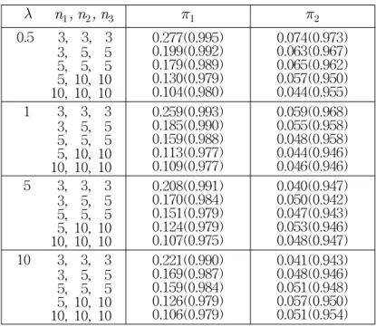
We evaluate the frequentist coverage probability by investigating the credible interval of the marginal posteriors density of λ under the noninformative prior π given in Section 3 for several configurations

(λ, µ

₁

, , µ

_k

)

and

(n

₁

, , n

_k

)

. That is to say, the frequentist coverage of a (1

−

α )th posterior quantile should be close to 1

−

α. This is done numerically. Table 1 gives numerical values of the frequentist coverage probabilities of 0.05(0.95) posterior quantiles for the our prior.

The computation of these numerical values is based on the following algorithm for any fixed true

(λ, µ

₁

, , µ

_k

)

and any prespecified probability value α. Here α is 0.05(0.95). Let

θ

^π₁

(α│X)

be the

Table 1: Frequentist Coverage Probabilities of 0.05 (0.95) Posterior Quantiles for λ λ

n

₁

, n

₂

, n

₃

π

₁

π

₂ 0.5 3, 3, 3

3, 5, 5 5, 5, 5 5, 10, 10 10, 10, 10

0.277(0.995) 0.199(0.992) 0.179(0.989) 0.130(0.979) 0.104(0.980)

0.074(0.973) 0.063(0.967) 0.065(0.962) 0.057(0.950) 0.044(0.955) 1 3, 3, 3

3, 5, 5 5, 5, 5 5, 10, 10 10, 10, 10

0.259(0.993) 0.185(0.990) 0.159(0.988) 0.113(0.977) 0.109(0.977)

0.059(0.968) 0.055(0.958) 0.048(0.958) 0.044(0.946) 0.046(0.946) 5 3, 3, 3

3, 5, 5 5, 5, 5 5, 10, 10 10, 10, 10

0.208(0.991) 0.170(0.984) 0.151(0.979) 0.124(0.979) 0.107(0.975)

0.040(0.947) 0.050(0.942) 0.047(0.943) 0.053(0.946) 0.048(0.947) 10 3, 3, 3

3, 5, 5 5, 5, 5 5, 10, 10 10, 10, 10

0.221(0.990) 0.169(0.987) 0.159(0.984) 0.126(0.979) 0.106(0.979)

0.041(0.943) 0.048(0.946) 0.051(0.948) 0.057(0.950) 0.051(0.954)

posterior α-quantile of λ _given x. That is to say,

F (λ

^π

(α│

X

)│

X

) = α

_, where F ( │X) is the marginal posterior distribution of λ. Then the frequentist coverage probability of this one sided credible interval of λ _is

P

_(λ,µ

1, ,µk)

(α;λ ) = P

_(λ,µ

1, ,µk)

(0 < λ≤λ

^π

(α│X)).

(16) The estimated

P

_(λ,µ

1, ,µk)

(α;λ )

when α = 0.05 (0.95 ) is shown in Table 1 for the k = 3 case.

In particular, for fixed

(λ, µ

₁

, µ

₂

, µ

₃

)

, we take 5,000 independent random samples of X from the model (1). In our simulation, we take

(µ

₁

, µ

₂

, µ

₃

) = (1, 2, 3 ).

For the cases presented in Table 1, we see that the one-at-a-time reference prior

π

₂ matches the target coverage probability much more accurately than the Jeffreys' prior

π

₁ for small values of

n

₁,

n

₂ and

n

₃, and values of λ . Note that the one-at-a-time reference prior satisfies a second order matching criterion but the Jeffreys' prior is not matching prior. Thus we recommend to use the one-at-a-time reference prior

π

₂ in the sense of asymptotic frequentist coverage property.

In the inverse gaussian populations, we have found a prior which is a second order matching prior and reference prior for the common scale parameter. It turns out that the one-at-a-time reference prior satisfies the second order matching criterion. Also we revealed that the one-at-a-time reference prior is a joint probability matching prior for (λ, µ₁, µ₂, µ₃). Thus we recommend the use of the on-at-a-time reference prior for the Bayesian inference in the analysis of reciprocals and regression models.

References

1. Berger, J.O. and Bernardo, J.M. (1989). Estimating a Product of Means : Bayesian Analysis with Reference Priors. Journal of the American Statistical Association, 84, 200-207.

2. Berger, J.O. and Bernardo, J.M. (1992). On the Development of Reference Priors (with discussion). Bayesian Statistics IV, J.M.

Bernardo, et. al., Oxford University Press, Oxford, 35-60.

3. Bernardo, J.M. (1979). Reference Posterior Distributions for Bayesian Inference (with discussion). Journal of Royal Statistical Society, B, 41, 113-147.

4. Chhikara, R.S. and Folks, L. (1978). The Inverse Gaussian Distribution

and Its Statistical Application-A Review. Journal of Royal Statistical Society, B, 40, 263-289.

5. Chhikara, R.S. and Folks, L. (1989). The Inverse Gaussian Distribution;

Theory, Methodology and Applications, Marcel Dekker, New York.

6. Datta, G.S. (1996). On Priors Providing Frequentist Validity for Bayesian Inference for Multiple Parametric Functions. Biometrika, 83, 287-298.

7. Datta, G.S. and Ghosh, J.K. (1995a). On Priors Providing Frequentist Validity for Bayesian Inference. Biometrik, 8, 37-45.

8. Datta, G.S. and Ghosh, M. (1995b). Some Remarks on Noninformative Priors. Journal of the American Statistical Association, 90, 1357-1363.

9. Datta, G.S. and Ghosh, M. (1996). On the Invariance of Noninformative Priors. The Annals of Statistics, 24, 141-159.

10. Datta, G. S., Ghosh, M. and Mukerjee, R. (2000). Some New Results on Probability Matching Priors. Calcutta Statistical Association Bulletin, 50, 179-192.

11. DiCiccio, T.J. and Stern, S.E. (1994). Frequentist and Bayesian Bartlett Correction of Test Statistics based on Adjusted Profile Likelihood.

Journal of Royal Statistical Society, B, 56, 397-408.

12. Fries, A. and Bhattacharyya, G.K. (1983). Analysis of Two-Factor Experiments under an Inverse Gaussian Model. Journal of the American Statistical Association, 78, 820-826.

13. Ghosh, J.K. and Mukerjee, R. (1992). Noninformative Priors (with discussion). Bayesian Statistics IV, J.M. Bernardo, et. al., Oxford University Press, Oxford, 195-210.

14. Mukerjee, R. and Ghosh, M. (1997). Second Order Probability Matching Priors. Biometrika, 84, 970-975.

15. Mukerjee, R. and Reid, N. (1999). On A Property of Probability Matching Priors:Matching the Alternative Coverage Probabilities.

Biometrika, 86, 333-340.

16. Seshadri, V. (1999). The Inverse Gaussian Distribution: Statistical Theory and Applications, Springer, New York.

17. Stein, C. (1985). On the Coverage Probability of Confidence Sets based on a Prior Distribution. Sequential Methods in Statistics, Banach Center Publications, 16, 485-514.

18. Tibshirani, R. (1989). Noninformative Priors for One Parameter of Many. Biometrika, 76, 604-608.

19. Tweedie, M.C.K. (1957a). Statistical Properties of Inverse Gaussian Distributions I. The Annals of Mathematical Statistics, 28, 362-377.

20. Tweedie, M.C.K. (1957b). Statistical Properties of Inverse Gaussian Distributions II. The Annals of Mathematical Statistics, 28, 696-705.

21. Welch, B.L. and Peers, H.W. (1963). On Formulae for Confidence Points

based on Integrals of Weighted Likelihood. Journal of Royal Statistical Society, B, 25, 318-329.

22. Whitmore, G.A. (1979). An Inverse Gaussian Model for Labour Turnover. Journal of Royal Statistical Society, A, 142, 468-478.

[ received date : Aug. 2004, accepted date : Nov. 2004 ]