Efficient Meshfree Analysis Using Stabilized Conforming Nodal Integration for Metal Forming Simulation
Kyu-Taek Han†
(Received August 17, 2010; Revised October 5, 2010; Accepted October 12, 2010)
Abstract:An efficient meshfree method based on a stabilized conforming nodal integration method is developed for elastoplastic contact analysis of metal forming processes. In this approach, strain smoothing stabilization is introduced to eliminate spatial instability in Galerkin meshfree methods when the weak form is integrated by a nodal integration. The gradient matrix associated with strain smoothing satisfies the integration constraint for linear exactness in the Galerkin approximation. Strain smoothing formulation and numerical procedures for path-dependent problems are introduced. Applications of metal forming analysis are presented, from which the computational efficiency has been improved significantly without loss of accuracy.
Key words:Stabilized conforming, Efficient meshfree method, Nodal integration, Metal forming
†Corresponding Author(Department of Mechanical Engineering, Pukyong National University, E-mail:[email protected], Tel: 051-629-6135)
1. Introduction
Meshfree methods can be classified collectively as a Galerkin meshfree method[1-5], a Petrov-Galerkin meshfree method[6-7], or a collocation meshfree method[8-10]. Gauss integration is commonly used in Galerkin meshfree methods for integration of weak form. Due to the complexity involved in Gauss integration for Galerkin meshfree methods, attempts have been made to develop nodal integration methods for meshfree computation.
The objective of this study is to develop a stabilized conforming nodal integration (SCNI) for the Galerkin meshfree method to achieve higher efficiency with desired
accuracy and convergent properties. A strain smoothing stabilization is used to compute nodal strain by a divergence counterpart of a spatial averaging of strain. This strain smoothing avoids evaluating derivatives of meshfree shape functions at nodes and thus eliminates spurious modes. That is, in this study, a strain smoothing stabilization is implemented as a means to meet integration constraints and to provide a stabilization for nodal integration. SCNI not only yields a significant reduction in computational cost, it can also achieve a higher accuracy[1] due to the satisfaction of integration constraints. In this paper, the history-dependent problems with
applications to metal forming problems are investigated and also several metal forming problems are demonstrated.
2. Stabilized conforming nodal integration
2.1 Meshfree shape function
The approximation methods most widely used in meshfree methods are the moving least-squares(MLS) approximation, partition of unity method (PUM), and the reproducing kernel (RK) approximation[7]. Without loss of generality, the MLS and RK approximation for construction of the meshfree shape function is introduced in this section. The reproducing MLS-RK approximation of a variable u(x), denoted by , is
∑ (1)
(2)
∑ (3) where is a kernel function with compact support “”, dI is the coefficient of approximation(generally not a nodal value),
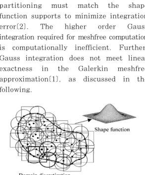
is the vector of monomial basis, NP is the number of particles, and is the meshfree shape function. A meshfree shape function and domain discretization is illustrated in Figure 1. This meshfree shape function was constructed based on reproducing conditions and therefore is capable of exactly representing nth order monomials (th order consistency):∑ ≤ ≤ (4)
The meshfree Galerkin approximation is formulated by introducing meshfree shape functions, e.g., Eq. (2), into the weak form. Gauss integration is usually used in the integration of the weak form. It has become apparent that shortcomings exist with respect to Gauss integration for Galerkin meshfree methods.
Using Gauss integration, domain partitioning must match the shape function supports to minimize integration error[2]. The higher order Gauss integration required for meshfree computation is computationally inefficient. Further, Gauss integration does not meet linear exactness in the Galerkin meshfree approximation[1], as discussed in the following.
Figure 1: Meshfree discretization and shape function.
2.2 Integration constraints and strain smoothing stabilization
To obtain linear exactness in the Galerkin approximation, a discrete linear displacement must exactly satisfy the discrete equilibrium equation of a boundary value problem in which the solution is linear. Linear exactness in Galerkin approximation first requires linear consistency in the MLS-RK approximation. Second, numerical integration of stiffness and force must meet the following condition for interior nodes[1].
for all interior nodes {∩ } (5) where is the gradient matrix associated with node I, is the total boundary, is the integration point, is the weight, and NIT is the number of integration points. For shape functions intersect with essential boundary, flux equilibrium is required[3]. Strain smoothing stabilization has been proposed [1] to achieve two objectives: (1) to avoid taking derivatives at nodal points for stability, and (2) to construct a modified gradient matrix that satisfies the integration constraints in Eq. (5). A strain smoothing equation has been proposed by[1] as:
(6)
Introducing shape function for displacement into Eq. (6) leads to
∈
(7)
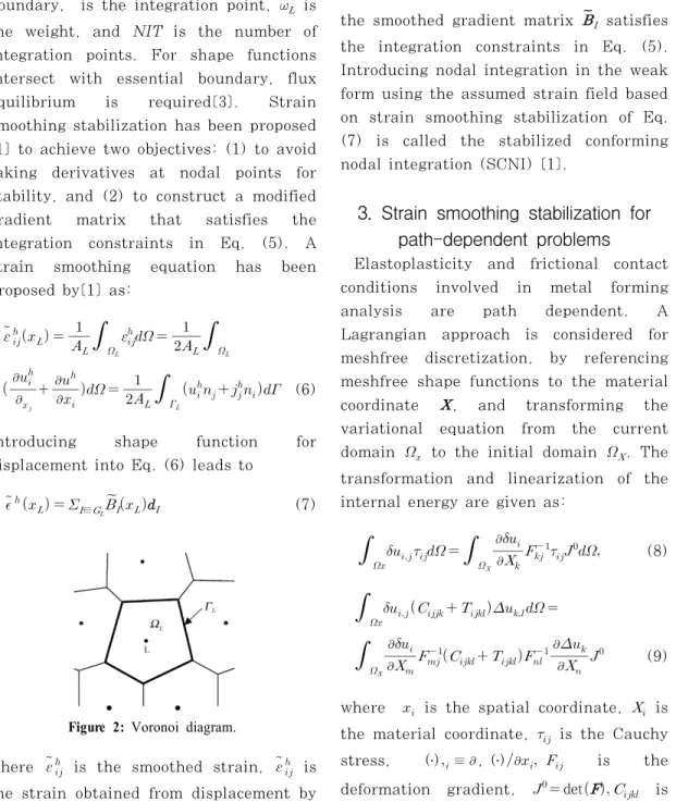
Figure 2: Voronoi diagram.
where is the smoothed strain, is the strain obtained from displacement by
compatibility, , and
are the representative domain and boundary, respectively, of node L obtained from, for example, the Voronoi diagram in Figure 2, and is the area (or volume) of . It can be shown that the smoothed gradient matrix satisfies the integration constraints in Eq. (5).
Introducing nodal integration in the weak form using the assumed strain field based on strain smoothing stabilization of Eq.
(7) is called the stabilized conforming nodal integration (SCNI) [1].
3. Strain smoothing stabilization for path-dependent problems
Elastoplasticity and frictional contact conditions involved in metal forming analysis are path dependent. A Lagrangian approach is considered for meshfree discretization, by referencing meshfree shape functions to the material coordinate , and transforming the variational equation from the current domain to the initial domain . The transformation and linearization of the internal energy are given as:
(8)
(9)
where is the spatial coordinate, is the material coordinate, is the Cauchy stress, (․)≡ , (․) is the deformation gradient, det is
the material response tensor, and is the initial stress tensor. To employ a stabilized conforming nodal integration in the evaluation of stiffness and internal force, the deformation gradient is smoothed by
≡
(10a)
(10b) where , and are the surface normal, the nodal representative domain and boundary at node L, respectively, at the initial configuration, and
.
Introducing a Lagrangian shape function
for displacement ∑
into Eq. (10) yields
∑, (11)
Where
(12) For path-dependent problems, the computation of spatial derivatives of displacement is required for stress update. Using the Lagrangian approach, stress update is computed using a smoothed strain increment
(13)
where is the inverse of computed by Eq. (10). To introduce smoothed deformation gradient as an independent variable, the mixed
variational equation is formulated by an assumed strain method:
∏
(14) Applying similar procedures to the incremental variational equation of Eq.
(9), the resulting stiffness matrix and force vector can be obtained as:
(15)int ∑
(16)
(17)
(18)
(19)
det (20)
Where is the gradient matrix associated with the smoothed deformation gradient given in Eqs. (10a)-(10b), and
is the Cauchy stress calculated using the smoothed strain. Using the Lagrangian approach, the value of evaluated at the material integration point does not change with the
material deformation, and can therefore be stored and reused for computing
and int in each load step. For contact problems, contact constraints are introduced through a penalty-type perturbed Lagrangian formulation [5]. Collocation is employed in the boundary integration of contact stiffness and force terms. A smooth contact surface representation is introduced to generate a smooth contact surface through the nodal locations of the set of contact surface nodes. The smooth surface representation is incorporated into the meshfree formulation to yield a consistent tangent operator for frictional contact problems.
4. Numerical examples
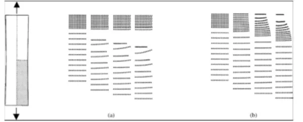
4.1 Necking
An axisymmetric elastoplastic bar is subjected to an axial prescribed displacement as shown in Figure 3. A geometric imperfection at the center of the rod is introduced, for which a quarter of the geometry is modeled. The displacement solution from direct nodal integration exhibits spatial oscillation in both the axial and transverse directions.
Non-physical necking deformation occurs near the interface of the regions that
Figure 3: Necking analysis results after (a) direct nodal integration and (b)stabilized conforming nodal integration.
exhibit substantial difference in nodal density (Figure 3(a)). Spatial instability and non-physical necking are suppressed and corrected by the SCNI (Figure 3(b)).
4.2 Stretch forming
The problem is described as shown in Figure 4. A plane-strain sheet metal is stretched by a cylindrical punch. Because of symmetry, only half of the total geometry is modeled. When direct nodal integration is used without stabilization, spurious modes occur in both membrane and transverse directions, as shown in Figure 5(a). These unstable modes are eliminated in the SCNI technique, as illustrated in Figure 5(b).
Figure 4: Cylindrical punch problem.
Figure 5: The four modes of stiffness constructed using direct and SC nodal integrations (a) direct nodal integration and (b) stabilized conforming nodal integration
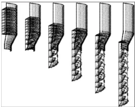
4.3 Extrusion
A 3D elastoplastic cylindrical billet is extruded through a rigid circular die as shown in Figure 6. Extrusion is achieved
by prescribing displacements at the top end of the billet. Because of symmetry, only one quarter of the total billet is modeled by 711 particles. Both the Gauss integration method and the proposed stabilized conforming nodal integration were used in the analysis for comparison.
The SCNI method yields results very similar to that of the Gauss integration, and therefore only the deformation obtained by SCNI is shown in Figure 7.
The CPU time for SCNI is only 10% of that required in the Gauss integration method.
Figure 6: Geometry of extrusion problem.
Figure 7: Extrusion processes modeled by stabilized conforming nodal integration.
4.4 Beam subjected to a shear load
The accuracy and convergence in regular and irregular discretization of a beam problem using integration methods are studied. The problem statement and boundary conditions of the beam problem
are given in Figure 8.
Figure 8: Problem statement of beam subjected to a shear load.
Three regularly refined meshfree discretizations for a half-model (anti-symmetry) are shown in Figure 9.
Figure 9: Regular discretization and refinement of half beam.
Linear basis functions and a normalized support size of 2.01 are used in regular discretizations. Superior performance of the stabilized conforming (SC) nodal integration over the direct nodal integration and Gauss integration methods is presented in the accuracy comparison of tip displacements in Table1. The direct nodal integration method displays a poor performance in the coarse model. SC nodal integration is particularly advantageous when a coarse model is used.
Table 1: Comparison of tip displacement accuracy(%).
Discrete
model 5×5 Gauss int. Direct
nodal int SC nodal int.
63 nodes 124 nodes 205 nodes
93.4256 96.9630 98.2768
83.6453 91.9689 95.3838
97.3410 99.0507 99.5141
The solution of the direct nodal integration presents lower accuracy than that obtained from Gauss integration. SC nodal integration not only enhances accuracy of the direct nodal integration;
the method performs better than the Gauss integration method. Larger error near the boundary is observed in the solution of the direct nodal integration, whereas Gauss integration and SC nodal integration methods generate similar results. In Figure 10, several refinements of an irregular model are constructed to study the performance of integration methods in irregular discretization. A Voronoi diagram for nodal integration methods is also plotted in Figure 10.
Figure 10: Irregular discretization, refinement, and Voronoi diagram.
The shape function support size in this study is increased slightly so that a normalized support size with respect to the maximum nodal distance is 2.01 in each model. Note that since support size is kept constant for all shape functions, the normalized support sizes in dense areas are higher than 2.01. Due to the slight irregularity in the discretization, the tip displacement accuracy of direct nodal integration methods reduces slightly. Surprisingly, the accuracy of SC nodal integration increases slightly compared to that of the regular case.
This is probably due to the small increase in normalized support size in the dense areas compared to the regular model. The
displacement distribution further confirms the effectiveness of SC nodal integration.
5. Conclusions
A stabilization technique for nodally integrated Galerkin meshfree methods for path-dependent problems has been developed to enhance computational efficiency in meshfree analysis. The proposed strain smoothing in the deformation gradient results in a smoothed gradient matrix that meets the linear exactness in the Galerkin approximation and it also serves as a stabilization mechanism. It has shown that a severe oscillation in displacement occurs in the solution using the direct nodal integration which was effectively suppressed with using of the proposed stabilized conforming nodal integration.
In this approach, the formation of the discrete equations was accelerated by an order of magnitude compared to the Gauss integration method. Particularly, substantial memory savings were achieved particularly, for path-dependent materials. Several metal forming problems were analyzed to examine the effectiveness of the proposed method.
Also in this study, although a Voronoi diagram is used for obtaining representative nodal domain and the associated weights for the stabilized conforming nodal integration, other methods can also be used for this purpose.
References
[1] S. Yoon, Y. You, “A stabilized conforming nodal integration for
Galerkin meshfree methods”, Int. J.
Numer. Meth. Eng., vol.50, pp. 435–
466, 2001.
[2] J. Dolbow, T. Belytschko, “Numerical integration of Galerkin weak form in meshfree methods”, Comput. Mech., vol.23, pp. 219–230, 1999.
[3] T. Belytschko, Y.Y. Lu, L. Gu,
“Element-free Galerkin methods”, Int.
J. Numer. Meth. Eng., vol.37, pp. 229 –256, 1994.
[4] S. Beissel, T. Belytschko, “Nodal integration of the element-free Galerkin method”, Comput. Methods Appl. Mech. Eng., vol. 139, pp. 49-74, 1996.
[5] T. Belytschko, Y. Krongauz, M.
Fleming, D. Organ, W.K. Liu, “ Smoothing and accelerated computations in the element-free Galerkin method”, J. Comput. Appl.
Math., vol. 74, pp. 111-126, 1996.
[6] C. Pan, C.M.O.L. Roque, H.P. Wang,
“A Lagrangian reproducing kernel particle method for metal forming analysis”, Comput. Mech., vol.22, pp.
289–307, 1998.
[7] W.K. Liu, S. Jun, Y.F. Zhang,
“Reproducing kernel particle methods”, Int. J. Numer. Meth. Fluids, vol.20, pp. 1081–1106, 1995.
[8] C.A.M. Duarte, J.T. Oden, “A h–p adaptive method using clouds”, Comput. Methods Appl. Mech. Eng., vol.139, pp. 237–262, 1996.
[9] G.R. Liu, Z.H. Tu, “ An adaptive procedure based on background cells for meshless methods”, Comput. Meth.
Appl. Mech. Eng. vol.191, pp. 1923–
1943, 2002.
[10] D. Wang, J.S. Chen, “Locking-free stabilized conforming nodal integration for meshfree Mindlin-Reissner plate formulation”, Comput. Meth. Appl.
Mech. Eng., vol.193, pp. 1065-1083, 2004.
Author Profile
Kyu-Taek Han
He received the B.E. and M.E. degree in Mechanical Engineering from Busan National University in 1982 and 1984 respectively. He received Ph.D. degree in Mechanical Engineering from Busan National University in 1988. He is currently a professor in Department of Mechanical Engineering at Pukyong National University in Busan. His research interests include computer aided analysis, meshfree method and computer aided manufacturing.