Multivariate Outlier Removing for the Risk Prediction of Gas Leakage based Methane Gas
Khongorzul Dashdondov1, Mi-Hye Kim2*
1Post-Doctor, Department of Computer Engineering, Chungbuk National University
2Professor, Department of Computer Engineering, Chungbuk National University
메탄 가스 기반 가스 누출 위험 예측을 위한 다변량 특이치 제거
홍고르출1, 김미혜2*
1충북대학교 컴퓨터공학과 박사, 2충북대학교 컴퓨터공학과 교수
Abstract In this study, the relationship between natural gas (NG) data and gas-related environmental elements was performed using machine learning algorithms to predict the level of gas leakage risk without directly measuring gas leakage data. The study was based on open data provided by the server using the IoT-based remote control Picarro gas sensor specification. The naturel gas leaks into the air, it is a big problem for air pollution, environment and the health. The proposed method is multivariate outlier removing method based Random Forest (RF) classification for predicting risk of NG leak. After, unsupervised k-means clustering, the experimental dataset has done imbalanced data. Therefore, we focusing our proposed models can predict medium and high risk so best. In this case, we compared the receiver operating characteristic (ROC) curve, accuracy, area under the ROC curve (AUC), and mean standard error (MSE) for each classification model. As a result of our experiments, the evaluation measurements include accuracy, area under the ROC curve (AUC), and MSE; 99.71%, 99.57%, and 0.0016 for MOL_RF respectively.
Key Words : Natural, Gas, Leak prediction, Random Forest, Multivariate Outlier Detection, LN transform .
요 약 본 연구에서는, 천연가스(NG) 데이터와 가스 관련 환경 요소 간의 관계를 기계학습 알고리즘을 사용하여 가스 누출 데이터를 직접 측정하지 않고 가스 누출 위험 수준을 예측하였다. 이번 연구는 서버가 제공하는 오픈 데이터인 IoT 기반 원격 제어 피카로(Picarro) 가스 센서 사양을 기반으로 사용했다. 천연 가스는 공기 중으로 누출이 되며, 대기 오염, 환경, 그리고 건강에 큰 문제가 된다. 본 연구에서 제안하는 방법은 천연 가스의 누출 위험 예측을 위한 랜덤 포레스트(Random Forest) 분류 기반 다변량 특이치 제거 방법이다. 비지도 k-평균 클러스터링 후에 실험 데이 터 집합은 불균형 데이터이다. 따라서 우리는 제안된 모델이 중간과 높은 위험 수준을 가장 잘 예측할 수 있다는 점에 초점을 맞춘다. 이 경우 각 분류 모델에 대한 수신자 조작 특성(ROC) 곡선, 정확도, 평균 표준 오차(MSE)를 비교했다.
실험 결과로 정확도, 수신자 조작 특성의 곡선 아래 영역(AUC, Area Under the ROC Curve), MSE가 각각 MOL_RF 의 경우 99.71%, 99.57%, 및 0.0016의 결과 값을 얻었다.
주제어 : 천연 가스, 누출 예측, 랜덤 포레스트, 다변량 특이치 검출, LN 변환
*This research was financially supported by the Ministry of Trade, Industry, and Energy (MOTIE), Korea, under the “Regional Specialized Industry Development Program (R&D, P0002072)” supervised by KIAT.
*Corresponding Author : Mi-Hye Kim([email protected]) Received October 30, 2020
Accepted December 20, 2020 Revised Novermber 27, 2020
Published December 28, 2020
1. Introduction
A gas leak has had a serious impression on environmental pollution and health. Therefore, it is important to predict the level of risk related to gas leakage. Recent studies aim to predict leakage of natural gas and beware of such potential accidents in advance.
The researchers have studied a pilot project of this mapping to explore the first step in gaining a better understanding of the effects of NG leaks in [1,2]. NG mass was measured using a Picarro CH4 sensor specification and a Google Street View machine in [3]. It is a gas sensor, fire-resistant, wired, and wireless transmitter that can be used in high-sensitivity facilities. In addition, this vehicle is an IoT-based remote monitoring system, a dual-antenna diagnostic solution used for real-time data aggregation analysis [4-7]. Further, we present a list of environmental and gas features raw data properties of NG found in mobile device-based methane gas studies from [15]. When NG is released into the air, it creates huge problems for the climate and the environment. The order of fluctuations in the sensitivity of the device used to measure the CH4 level was higher. The related work of this study is [8], there, used OrdinalEncoder (OE) normalization for the target feature of CH4 (g min). Then k-means clustering to the labeling of CH4 for the data pre-processing part. The flow rate of the CH4 leak is referred to in [1,2]. In recent years, a machine-based approach to environmental engineering has been widely used to predict natural gas leaks [4, 9]. They used factor analysis to reduce the size of the high-dimensional variables and to obtain the optical properties of the cluster analysis [10,11].
Standard, machine-learning techniques are divided into three categories as supervised, semi-supervised, and unsupervised. The data we use is unsupervised data without a label. The
purpose of this study was to compare the KNN, DT, RF, NB, and MLP [10, 12,13] classification techniques for feature selection using factor analysis (FA) and OE normalization for risk prediction of NG' leaks. The model is evaluated on the accuracy, mean squared error (MSE), AUC, and receiver operating characteristic curve (ROC). The main contributions of this research are, we propose the multivariate outlier removing Mahalanobis distance [13, 14] and OE based ML method to predict NG leakage risk detection in the open data by the unsupervised mode. In addition, after we performed a natural logarithmic (Ln) transformation, the overall content distribution pattern of the original data did not change significantly until the k-mean cluster analysis was performed. Therefore, our method is suitable for the early prediction of NG leaks in the air.
Therefore, in this study, based on the relationship between the gas data and the environmental elements assume by the gas were identified in order to predict the level of gas leakage risk without directly measuring the gas leak data.
2. Methodology
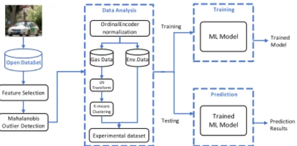
In this paper, we used Picaro's vehicle-based methane gas open data. Initially, we cleaned data for null and constant values row and column data. In this case, we selected 17 features from 33 features [18]. Fig. 1 shown the general system architecture of the proposed method. In this method, initially, we cleaning data by null and constant variables row and column and selected features. Behind feature selection, we removed outliers using multivariate outlier detecting Mahalanobis distance method. After outlier eliminating, we normalized data by the OrdinalEncoder technique [8]. As well, we divided data into two parts with the Gas and
Environment dataset. In the gas dataset, we converted by Ln transform. Furthermore, we using unsupervised k-means clustering algorithms for labeling into CH4 gas data. After labeling, we combined both data gas and environment by the labeled dataset. In this labeled dataset we make train machine learning models for predictive analysis. After the train, we had test predictive and evaluating models by accuracy measurement.
Open DataSet
Training
ML Model OrdinalEncoder
normalization
LN Transform
Data Analysis
Gas Data Env.Data
Experimental dataset
Trained ML Model
Prediction
Testing Training
Trained Model
Prediction Results K‐means
Clustering Feature Selection
Mahalanobis Outlier Detection
Fig. 1. The general system architecture of the proposed method
2.1 Mahalanobis Outlier Detection
Multivariate outliers can be identified with the use of Mahalanobis distance, which is the distance of a data point from the calculated centroid of the other cases where the centroid is calculated as the intersection of the mean of the variables being assessed. Each point is recognized as an X, Y combination and multivariate outliers lie a given distance from the other cases. The distances are interpreted using a p < 0.001 and the corresponding χ2 value with the degrees of freedom equal to the number of variables. Multivariate outliers can also be recognized using leverage, discrepancy, and influence. Leverage is related to Mahalanobis distance but is measured on a different scale so that the χ2 distribution does not apply. Large scores indicate the case if further out however may still lie on the same line. Discrepancy assesses the extent that the case is in line with the other cases. Influence is determined by leverage and discrepancy and assesses changes in
coefficients when cases are removed. Cases >
1.00 are likely to be considered the outliers.
It was introduced by Prof. P. C. Mahalanobis in 1936 and has been used in various statistical applications ever since. However, it’s not so well known or used in the machine learning practice.
1. It transforms the columns into uncorrelated variables
2. Scale the columns to make their variance equal to 1
3. Finally, it calculates the Euclidean distance.
The formula to compute Mahalanobis distance is as follows:
(1) where, is the square of the Mahalanobis distance, x is the vector of the observation (row in a dataset), m is the vector of mean values of independent variables (mean of each column), is the inverse covariance matrix of independent variables and (x – m) is essentially the distance of the vector from the mean, then divide this by the covariance matrix (or multiply by the inverse of the covariance matrix).
P value probability is shown as following equation
(2) In this paper, outliers are removed based on the Mahalanobis Distance for detection of multivariate outliers. We have 16 features for environments data and 1 feature for gas data, totally 17 features. There dependent variable is CH4, predictor variables are “CavityPressure”,
“CavityTemp”, “DasTemp”, “EtalonTemp”,
“WarmBoxTemp”, “OutletValve”, “GPS_ABS_LAT”,
“GPS_ABS_LONG”, “WS_WIND_LON”,
“WS_WIND_LAT”, “WS_COS_HEADING”,
“WS_SIN_HEADING”, “WIND_N”, “WIND_E”,
“WIND_DIR_SDEV”, “CAR_SPEED”.
In Fig. 2(a), outliers detected by Mahalanobis distance using a p < 0.001 and the corresponding χ2 value with the degrees of freedom. Fig. 2(b)
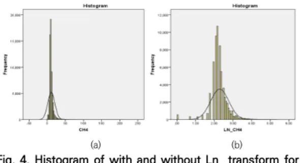
(a) (b)
Fig. 4. Histogram of with and without Ln transform for CH4. a) without Ln, b) with Ln.
shows removed outliers from dataset by rank p value. Where, degree of freedom has df=13.
Fig. 2. Comparison between before and after Mahalanobis outlier.
2.2 Ordinal Encoder
Encode categorical variables as an integer array. The input of this transformer is the same as an integer or string array and represents a value obtained by a category (discrete) characteristic. There converts feature to the ordinal integers. As a result, one integer column (0 to n-1) appears in one feature, and n is the number of categories. We implemented the OE normalization for all components. Fig. 3 shows plots of component 6 with and without OE.
Additionally, after OE, we transformed the log10 scale transform with all seven components. The results are shown in Fig. 4. It can be seen that the distribution of the initial values of the data mentioned in [1] is similar
(a) (b) Fig. 3. Plots of with and without OE normalization for
CH4 data. (a) with OE, (b) without OE.
After outlier detecting we have removed zero valued column as “GPS_ABS_LON_OE”, and after OE normalization we removed “CavityPressure”.
Now we have 14 features for environmental data.
Additionally, after OE, we transformed the Ln
scale transform with all features. Fig. 5 is the results before and after Ln transform of CH4 were compared. It can be seen that the distribution of the initial values of the data mentioned in [1] is similar.
(a) (b) Fig. 5. Comparison between before and after Ln
transform. (a) without Ln, (b) with Ln.
2.3 K-means Clustering
In this session we will explain one of the most popular ML unsupervised algorithm K-means clustering classification used to CH4 gas data.
The K-means is a multi-variable classification method developed by MacQueen in 1967 [11].
The main concept is to distribute the variables to the nearest class n values into k subgroups. The basic concept is to divide the variables into k subgroups of n values in the nearest class. We divided into three levels for gas leakage by low, medium, and high.
In Fig. 6, we illustrated k-means clustering results by the boxplot for CH4. Here final cluster center includes low, medium, and high reached 2.59, 3.65, and 4.48, respectively as almost the same with the [1] median threshold value (ppm) for defining elevated CH4. The cluster values
have as low-51582, medium-12104, and high-460. From the value of the clusters, it can be seen that the imbalanced data with CH4.
Fig. 6. Box plot of clusters for the gas data.
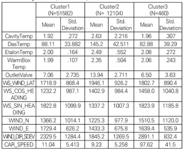
We also analyzed factors for depend variable is CH4 with other environment data. Table 2 shows descriptive statistics of features for CH4. Which is the cluster 1, 2, and 3 are low, medium and high. There have means and standard deviations of the features used in the factor analysis. The number of cases has N=69831.
Table 1. Descriptive Statistics of CH4 for Cluster Number of 1, 2, and 3 are used in the analysis phase (N=64146)
Cluster1
(N=51582) Cluster2
(N= 12104) Cluster3 (N=460) Mean Std.
Deviation Mean Std.
Deviation Mean Std.
Deviation
CavityTemp 1.92 .272 2.63 2.216 1.96 .307
DasTemp 88.11 33.882 145.2 42.511 82.88 39.29
EtalonTemp 2.00 .164 2.49 .552 2.08 .272
WarmBox
Temp 1.99 .107 2.35 .504 2.06 .243
OutletValve 7.06 2.735 13.94 2.711 6.50 3.63 WS_WIND_LAT 1718.9 868.4 1946.1 926.2 1802.7 890.4 WS_COS_HE
ADING 1232.2 987.1 1402.9 984.4 1458.0 1040.8 WS_SIN_HEA
DING 1822.8 1099.9 1337.2 1007.3 1823.9 1185.8 WIND_N 1366.2 1014.1 1225.3 977.9 1510.5 1120.0 WIND_E 1729.4 626.2 1433.3 675.8 1639.4 535.9 WIND_DIR_SDEV 2329.5 1284.4 1845.2 1269.5 2891.1 832.4 CAR_SPEED 11.04 5.413 9.23 5.258 97.62 41.5
Table 2 we can show communalities value for each clusters and extracted by PCA. From these results, it can be shown as the percentage of features of the value explained by the coefficient for the given variable. In other words, we obtain
indicating that about 87.0% of the variation in DasTemp_OE is explained by the cluster 1 factor model. Likewise, 81.6% in cluster 2, and 82.1% in cluster 3.
Extraction Cluster 1 Cluster 2 Cluster 3
CavityTemp_OE .400 .748 .549
DasTemp_OE .870 .816 .821
EtalonTemp_OE .781 .825 .851
OutletValve_OE .821 .766 .873
WS_WIND_LON_OE .896 .827 .904
WS_WIND_LAT_OE .572 .565 .624
WS_COS_HEADING_OE .630 .780 .769
WS_SIN_HEADING_OE .693 .683 .787
WIND_N_OE .069 .587 .277
WIND_E_OE .525 .601 .673
WIND_DIR_SDEV_OE .705 .759 .831
CAR_SPEED_OE .134 .241 .192
Table 2. Communalities of Factor model for each clusters (Initial = 1, Extraction Method:
Principal Component Analysis. Only cases for which Cluster Number of 1, 2 and 3 are used in the analysis phase.)
The results suggested the best job of explaining variation in DasTemp_OE, EtalonTemp_OE, OutletValve_OE, and WS_WIND_LON_OE reached 87.0%, 78.1%, 82.1%, and 89.6% for the first cluster of CH4; DasTemp_OE, EtalonTemp_OE, and WS_WIND_LON_OE reached 81.6%, 82.5%, and 82.7% for the second cluster of CH4;
DasTemp_OE, EtalonTemp_OE, OutletValve_OE, WS_WIND_LON_OE, and WIND_DIR_SDEV_OE reached 82.1%, 85.1%, 87.3%, 90.4%, and 83.1%
for the third cluster of CH4. We can to see values that are close to the initial value one. This model shows that most of the features of these variables are explained. In this case, the model is better for some variables than for others. The model explains DasTemp_OE, EtalonTemp_OE, OutletValve_OE, WS_WIND_LON_OE, and WIND_DIR_SDEV_OE are the best for CH4 features. In additionally, not bad for other variables such as CavityTemp_OE, WS_WIND_LAT_OE, WS_COS_HEADING_OE, WS_SIN_HEADING_OE, WIND_N_OE, WIND_E_OE, WIND_DIR_SDEV_OE, and CAR_SPEED. However, for other variables such as CAR_SPEED_OE, the
model does not work very well and only explains about 24% of the changes. This model extracted by PCA.
3. Evaluation Metrics
The performance evaluation of this paper was completed using accuracy, AUC, F1-score, and MSE. We can find precisions and recall as follows [4]:
(3) The F1 score is the harmonic mean of precision and recall as follows:
∙ ∙
(4) We have studied on the multi-class case, there the average of the F1-score of each class label with weighting depending on the average parameter as Eq. (4).
The accuracy is a measure of the degree for the nearness of calculated value to its actual value. Accuracy is the sum of true positive fraction and true negative fraction among all the test data as Eq. (5).
(5) In addition, one of our evaluated metrics is the mean squared error (MSE) for the predicted leaks to relative to actual values was used:
(6) with m and n being the number of observations, which m is the number of data and n is predicting NG. The X and Y being the actual and predicted values for the i, j - th data point, respectively.
4. Experimental Results
The dataset is selected on [1, 8, 15] experimental data which named as “03/15/2017-0.3/25/2017”
for Sample_Raw open data [6]. In the default setting of training (70%) and testing (30%) set.
The descriptive statistics for experimental data have described in the Table 3.
Table 3. Descriptive statistics of classes for experimental dataset
Class Total Train 70% Test 30%
Low 51582 36136 15446
Medium 12104 8462 3642
High 460 304 156
Total 64146 44902 19244
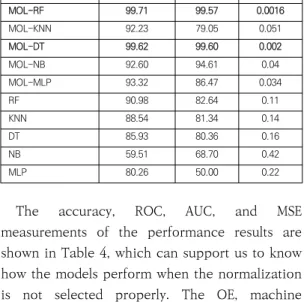
Table 4. Evaluation comparison of the proposed algorithms for experimental dataset(%).
Accuracy AUC MSE
MOL-RF 99.71 99.57 0.0016
MOL-KNN 92.23 79.05 0.051
MOL-DT 99.62 99.60 0.002
MOL-NB 92.60 94.61 0.04
MOL-MLP 93.32 86.47 0.034
RF 90.98 82.64 0.11
KNN 88.54 81.34 0.14
DT 85.93 80.36 0.16
NB 59.51 68.70 0.42
MLP 80.26 50.00 0.22
The accuracy, ROC, AUC, and MSE measurements of the performance results are shown in Table 4, which can support us to know how the models perform when the normalization is not selected properly. The OE, machine learning algorithms implemented in Python, and cluster analysis and Mahalanobis outlier detection removing implemented in SPSS 20.0.
The accuracy, AUC, MSE, and ROC curve measurements of the performance results are shown in Table 4, which can support us to know how the models perform when the normalization is not selected properly. The RF algorithm had the highest accuracy of 90.98%, AUC 82.64, MSE 0.11, and ROC 72.38% than other algorithms such as KNN, DT, NB, and MLP. We increased these performances by the Mahalanobis with OE and LN transform (MOL) model, and then the DNN model was improved by prediction
measurements. Our proposed MOL_RF has made accuracy, AUC, and MSE; 99.71%, 99.57%, and 0.0016 respectively. In addition, MOL_DT has made accuracy, AUC, and MSE; 99.62%, 99.60%, and 0.002 respectively.
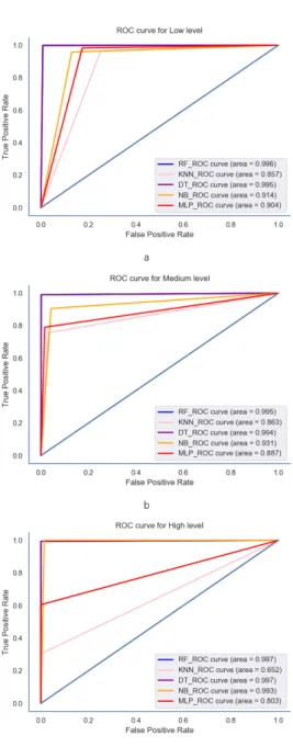
a
b
Fig. 7. Multi-class ROC curves by the compared F-OEc algorithms for low, medium and high levels. a) Low level class. b) Medium level class. c) High level class.
We provided multi-class ROC curves of compared some prediction model in Fig. 7. As mentioned before, we proposed to find a better model performance to predict medium and high-level classes for the experimental dataset.
The factor analysis with OE based RF shows higher ROC scores low-level 99.9%, medium-level 99.7%, and high-level 99.7% than others for all class level.
5. Conclusion
In this paper, we present relationship between NG data and environmental elements was performed using machine learning algorithms to predict the level of gas leakage risk without directly measuring gas leakage data on vehicle-based open data factor analysis. We eliminated outlier values using multivariate outlier detecting Mahalanobis distance method;
normalized them using the OrdinalEncoder, and then classified them using the k-mean cluster on the new CH4 value. We performed a Ln transformation, the overall content distribution pattern of the original data did not change significantly until the k-mean cluster analysis was performed. It is suggested to find a better model performance to predict the medium and high-levels for the unbalanced experimental data set. Our proposed MOL_RF methods predict the risk of leakage in the suggested algorithms, with accuracy, AUC, and MSE, reaching 99.71%, 99.57%, and 0.0016 respectively. In addition, MOL_DT has made accuracy, AUC, and MSE;
99.62%, 99.60%, and 0.002 respectively. The system has implemented the SPSS and Python, including its performance, is tested on open real data.
REFERENCES
[1] Z. D. Weller, D. K. Yang & J. C. Fischer. (2019). An open source algorithm to detect natural gas leaks from mobile methane survey data. PLOS ONE, 14(2), e0212287.
[2] V. N. Vapnik. (1995). The nature of statistical learning theory. New York: Springer.
[3] J. C. von Fischer & D. Cooley et. al. (2017). Rapid, Vehicle-Based Identification of Location and Magnitude of Urban Natural Gas Pipeline Leaks.
Environmental Science & Technology, 51(7), 4091-4099.
DOI: 10.1021/acs.est.6b06095.
[4] P. Xue, Y. Jiang, Z. Zhou, X. Chen, X. Fang & J. Liu.
(2020). Machine learning-based leakage fault detection for district heating networks. Energy and Buildings, 223, 110161,
DOI: 10.1016/j.enbuild.2020.110161.
[5] Y. M. Ju, H. S. Lee & J. C. Oh. (2018). Design and Implementation of Gas Leakage Alarm IoT System for Safety Helmet. ournal of the Korea Convergence Society,13(6), 1411–1416.
DOI: 10.13067/JKIECS.2018.13.6.1411.
[6] J. A. Lee & M. H. Kim. (2018). Gas Safety Monitoring App. Development Design for Gas Workers. Journal of the Korea Convergence Society, 9(10), 61–67.
DOI: 10.15207/JKCS.2018.9.10.061.
[7] J. A. Lee & M. H. Kim. (2017). Work Type Classification of Gas Safety Workers and Interaction Function Design for IoT-based App. Development, Journal of the Korea Convergence Society, 8(5), 45–
52. DOI: 10.15207/JKCS.2017.8.5.045.
[8] D. Khongorzul, M. H. Kim & S. M. Lee. (2019).
OrdinalEncoder based DNN for Natural Gas Leak Prediction. J. Korea Convergence Society, 10(10), 7-13.
[9] Y. Xu, X. Zhao, Y. Chen & Z. Yang. (2019). Research on a Mixed Gas Classification Algorithm Based on Extreme Random Tree. Appl. Sci., 9, 1728.
[10] S. B. Zhu, Z. L. Li, S. M. Zhang, L. L. Liang & H. F.
Zhang. (2018). Natural gas pipeline valve leakage rate estimation via factor and cluster analysis of acoustic emissions. Measurement, 125, 48-55.
DOI: 10.1016/j.measurement.2018.04.076
[11] D. Khongorzul, S. M. Lee, Y. K. Kim & M. H. Kim.
(2019). Image Denoising Methods based on DAECNN for Medication Prescriptions. Journal of the Korea Convergence Society, 10(5), 17–26.
DOI: 10.15207/JKCS.2019.10.5.017.
[12] M. Jupri & R. Sarno. (2018). Taxpayer compliance classification using C4.5, SVM, KNN, Naive Bayes and MLP. Int. Conf. on Inform. & Commun. Technology on
Proceedings, pp. 297-303. Yogyakarta.
[13] E. Cabana, R. E. Lillo & H. Laniado. (2019).
Multivariate outlier detection based on a robust Mahalanobis distance with shrinkage estimators. Stat Papers.
DOI: 10.1007/s00362-019-01148-1
[14] Q. Yan, J. Chen & L. D. Strycker. (2018). An Outlier Detection Method Based on Mahalanobis Distance for Source Localization. Sensors, 18(7), 2186.
DOI: 10.3390/s1807218.
[15] https://github.com/JVF-CSU/MobileMethaneSurveys/tr ee/master/Scripts/SampleRawData
홍 고 르 출(Khongorzul Dashdondov) [정회원]
․ 2000년 12월 : 몽골국립대학교 수학 과(이학사, 이학석사)
․ 2013년 8월 : 충북대학교 전파통신공 학과(공학박사)
․ 2017년 3월 ~ 현재 : 충북대학교 컴 퓨터공학과 연구원
․관심분야 : Probability and Statistics, Queueing theory, Image processing, Machine Learning, Deep Learning
․ E-Mail : [email protected]
김 미 혜(Mi-Hye Kim) [정회원]
․ 1992년 2월 : 충북대학교 수학과 (이 학사)
․ 1994년 2월 : 충북대학교 수학과 (이 학석사)
․ 2001년 2월 : 충북대학교 수학과 (이 학박사)
․ 2004년 9월 ~ 현재 : 충북대학교 컴 퓨터공학과 교수
․ 관심분야 : 빅데이터, 기능성 게임, 유비쿼터스 게임, 플랫폼, 퍼지측도 및 퍼지적분, 제스츄어 인식
․ E-Mail : [email protected]