2004, Vol. 15, No. 3, pp. 645∼654
Bayesian Test for the Intraclass Correlation Coefficient in the One-Way Random Effect Model
Sang Gil Kang1) ․ Hee Choon Lee2)
Abstract
In this paper, we develop the Bayesian test procedure for the intraclass correlation coefficient in the unbalanced one-way random effect model based on the reference priors. That is, the objective is to compare two nested model such as the independent and intraclass models using the factional Bayes factor. Thus the model comparison problem in this case amounts to testing the hypotheses H1:ρ = 0 versus H2:ρ≠0. Some real data examples are provided.
Keywords : Fractional Bayes Factor, Independent Model, Intraclass Model, Reference Prior
1. INTRODUCTION
Consider an unbalanced one-way random effect model
Yij= μ +αi+ εij, for i = 1, …, m and j = 1, …, ni, (1)
where μ is an unknown constant, and the αi and εij are independent normal variables with 0 means and variances σ2α and σ2, respectively. The testing for intraclass correlation coefficient ρ = σ2α/(σ2α+ σ2) is of interest.
The intraclass correlation coefficient and the ratio of variance components in the random effect model has been of interest for a long time, especially in animal
1) First Author : Assistant Professor, Department of Applied Statistics, Sangji University, Wonju, 220-702, Korea
E-mail : [email protected]
2) Professor, Department of Applied Statistics, Sangji University, Wonju, 220-702, Korea E-mail : [email protected]
of a certain trait of livestock breeders (Graybill et al., 1956). One difficult part of the analysis of the model (1) from the sampling theory of view is the possible negative estimates for σ2α as well as for σ2α/σ2. Thus a Bayesian analysis for this model is desirable, not only because of its intrinsic merit, but also because its ability to resolving this problem. Also the intraclass correlation ρ = σ2α/(σ2α+ σ2) is one-to-one transformation of φ = σ2α/σ2.
The problem of estimating intraclass correlation and the ratio of variance components in the one-way random effect model has been investigated by many authors from the Bayesian point of view. We may refer to Hill (1965), Box and Tiao (1973), Donner (1986), Palmer and Broemeling (1990), among others. For balanced one-way random effect model, Ye (1994) developed the reference priors for φ, examined frequentist coverage probabilities for various φ and compared risk functions of the Bayes estimators for the reference priors. Kim, Kang and Lee (2001) provided a class of second order probability matching priors for φ and ρ.
It is shown that among all of the reference priors, the one-at-a-time reference prior satisfies a second order matching criterion. For the unbalanced random effect model, Datta, Ghosh and Kim (2002) developed the first order probability matching prior for φ. In this case, the second order probability matching prior does not exist.
In Bayesian testing problem, the Bayes factor under proper priors or informative priors have been very successful. However, limited information and time constraints often require the use of noninformative priors. Since noninformative priors such as Jeffreys' priors or reference priors (Berger and Bernardo, 1989, 1992) are typically improper so that such priors are only defined up to arbitrary constants which affects the values of Bayes factors. Spiegalhalter and Smith (1982), O'Hagan (1995) and Berger and Pericchi (1996) have made efforts to compensate for that arbitrariness.
Berger and Pericchi (1996) introduced the intrinsic Bayes factor using a data-splitting idea, which would eliminate the arbitrariness of improper priors.
O'Hagan (1995) proposed the fractional Bayes factor. For removing the arbitrariness he used to a portion of the likelihood with a so-called the fraction b.
These approaches have shown to be quite useful in many statistical areas.
The present paper focuses on Bayesian testing procedure for the intraclass correlation coefficient in the unbalanced one-way random effect model. For dealing Bayesian testing for the intraclass correlation coefficient in the unbalanced one-way random effect model, we use the fractional Bayes factor (O'Hagan, 1995).
The outline of the remaining sections is as follows. In Section 2, using the reference priors, we provide the Bayesian testing procedure based on the fractional Bayes factor. In Section 3, some real examples are given.
2. BAYESIAN TEST PROCEDURES
2.1 Preliminaries
Models (or Hypotheses) H1, H2, …, Hq are under consideration, with the data x = ( x1,x2, … ,xn) having probability density function fi( x ∣ θi) under model Hi,i= 1,2,…,q. The parameter vectors θi are unknown. Let πi( θi) be the prior distribution of model Hi, and let pi be the prior probabilities of model Hi,
i = 1,2,…,q. Then the posterior probability that the model Hi is true is
P( Hi∣ x ) =(∑j = 1q ppji ⋅B ji)- 1, (1) where Bji is the Bayes factor of model Hj to model Hi defined by
Bji= mj( x ) mi( x ) =
⌠⌡fj( x ∣ θj)πj( θj)d θj
⌠⌡fi( x∣ θi)πi( θi)d θi . (2) The Bji interpreted as the comparative support of the data for the model j to i. The computation of Bji needs specification of the prior distribution πi( θi) and πj( θ). Usually, one can use the noninformative prior, often improper, such as uniform prior, Jeffreys prior, reference prior or probability matching prior. Denote it as πNi. The use of improper priors πNi(⋅) in (2) causes the Bji to contain unspecified constants. To solve this problem, O'Hagan (1995) proposed the fractional Bayes factor for Bayesian testing and model selection problem as follow.
When the πNi( θi) is noninformative prior under Hi, equation (2) becomes
BNji=
⌠⌡fj( x ∣ θj)πNj( θj)d θj
⌠⌡fi( x∣ θi)πNi( θi)d θi .
Then the fractional Bayes factor of model Hj versus model Hi is
BFji= BNji⋅
⌠⌡fbi( x ∣ θi)πNi( θi)d θi
⌠⌡fbj( x∣ θj)πNj( θj)d θj = BNji⋅ mb1( x) mb2( x) ,
fi( x ∣ θi) is the likelihood function and b specifies a fraction of the likelihood which is to be used as a prior density. He proposed three ways for the choice of the fraction b. One frequently suggested choice is b = m/n, where m is the size of the minimal training sample, assuming this is well defined. (see O'Hagan, 1995, 1997 and the discussion by Berger and Mortera of O'Hagan, 1995).
2.2 Bayesian Model Selection using Fractional Bayes Factor
In the unbalanced one-way random effect model, the intraclass correlation coefficient is given by ρ = σ2α/(σ2α+ σ2). We want to test the hypotheses H1:ρ = 0 versus H2:ρ≠0. That is, we compare two nested models such as independent and intraclss model. In this hypothesis testing problem, our objective is to develop a Bayesian test based on the fractional Bayes factors under the reference priors.
Under the hypothesis H1, the model is the independent model. Thus the likelihood function of parameters ( μ, σ2) is given by
L( μ,σ2) = ( 1
2π )N/2σ- Nexp { - 1
2σ2 [S2+ ∑m
i = 1ni( yi- μ)2] }, where S2= ∑m
i = 1∑
ni
j= 1(yij- yi)2, yi=∑
ni
j= 1y ij/ni and N = ∑m
i = 1∑
ni
j= 1ni. And the reference prior for μ and σ2 is given by
π1(μ,σ2) ∝ σ - 2.
Then the element of fractional Bayes factor under M1 is given by
mb1( y ) = ⌠⌡
∞ 0
⌠⌡
∞
- ∞Lb(μ,σ2∣ y )π1(μ,σ2)dμdσ2
= π-
Nb - 1
2 N -
1 2b-
Nb
2 Γ(Nb - 1
2 )[∑
m i = 1∑
ni
j = 1y2ij- N y2] -
Nb - 1
2 ,
where y = ∑m
i = 1∑
ni
j = 1y ij/N .
For the hypothesis H2, the model becomes intraclass model. In this case, the reference prior developed by Datta, Ghosh and Kim (2002). This prior is given by
π2(θ1, θ2, θ3)
∝ ( 1 - θ1)- 2θ- 12 {∑m
i = 1n2i(1+ niθ1
1 - θ1 )- 2- 1 N [∑m
i = 1ni(1 + niθ1
1- θ1 )- 1]2}
1 2,
where θ1= σ2α/(σ2+ σ2α), θ2= σ2[∏
m
i = 1(σ2+ niσ2α)/σ2] 1/N and θ3= μ. The expression of original parametrization of this prior is convenient for the computation of the marginal distribution. So in original parametrization ( μ,σ2α, σ2), the reference prior for μ, σ2α and σ2 is given by
π2(μ,σ2α, σ2) ∝ σ- 4[∑
m i = 1
n2iσ4
(σ2+ niσ2α)2 - 1 N (∑
m i = 1
niσ2
σ2+ niσ2α )2] 1/2. And the likelihood function is
L( μ,σ2α,σ2) = ( 1
2π )N/2σ- N ∏m
i = 1( σ2+ niσ2α σ2 )-
1 2
× exp {- 1
2σ2 [S2+∑m
i = 1
niσ2
σ2+ niσ2α ( yi- μ)2] }.
Thus the element of fractional Bayes factor under H2 gives as follows.
mb2( y ) = ⌠⌡
∞ 0
⌠⌡
∞ 0
⌠⌡
∞
- ∞Lb(μ , σ2α, σ2∣ y )π2(μ, σ2α,σ2)dμdσ2αdσ2
= π -
Nb - 1 2 b-
Nb
2 Γ( Nb - 1
2 )T( y ;b), where
T( y ;b)
= ⌠⌡
∞ 0 (∑m
i = 1
ni 1+ niθ ) -
1 2 ∏m
i = 1(1+ niθ)-
b
2[S2+ ∑m
i = 1
ni
1+ niθ ( yi2- μ2θ)] -
Nb - 1 2
× [∑
m i = 1
n2i
(1+ niθ)2 - 1 N (∑
m i = 1
ni 1+ niθ )2]
1 2dθ,
where μθ= ( ∑
m i = 1
niyi
1+ niθ )/(∑
m i = 1
ni
1+ niθ ). Therefore the BN21 is given by
BN21= N
1
2T( y ;1) [∑
m i = 1∑
ni
j= 1y2ij- N y2] -
N - 1 2
.
Moreover
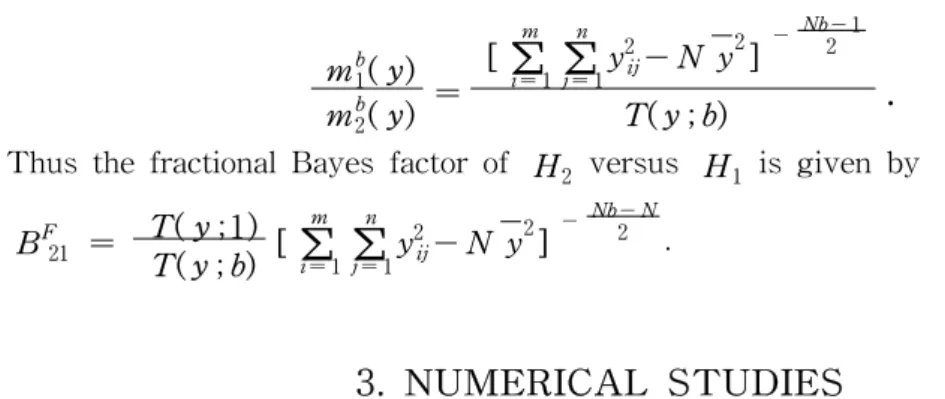
mb1( y ) mb2( y ) =
[∑
i = 1∑
j= 1y2ij- N y2] 2 N
1
2T( y ;b)
.
Thus the fractional Bayes factor of H2 versus H1 is given by
BF21 = T( y ;1) T( y ;b) [ ∑m
i = 1∑
ni
j= 1y2ij- N y2]-
Nb - N 2 .
Note that the calculation of the fractional Bayes factor of H2 versus H1 is requires an one dimensional integration.
Remark 1. In the balanced one-way random effect model, the element of fractional Bayes factor under H1 is given by
mb1( y ) = π -
Nb - 1
2 N -
1 2b-
Nb
2 Γ( Nb - 1
2 )[∑
m i = 1 ∑
n
j = 1y2ij- N y2]-
Nb - 1
2 ,
where y = ∑m
i = 1 ∑n
j = 1yij/N and N = mn . For H2, the reference prior is given by π2(μ,σ2α, σ2) ∝ σ- 2(σ2+ n σ2α)- 1.
This reference prior satisfies a second order matching criterion (Kim, Kang and Lee, 2001). Therefore the element of fractional Bayes factor under H2 gives as follows.
mb2( y ) = π-
Nb - 1
2 N -
1 2b-
Nb
2 Γ( Nb - 1
2 )T( y ;b), where
T( y ;b) = ⌠⌡
∞
0 (1+ n θ) -
mb - 1 2 - 1
[S21+ n
1 + nθ S22]-
Nb - 1
2 dθ.
Here S21= ∑m
i = 1 ∑n
j = 1(yij- yi)2, y i= ∑n
j = 1yij/n and S22= ∑m
i = 1( yi- y )2, y = ∑m
i = 1∑n
j = 1yij/N . Therefore the BN21 is given by
BN21= T( y ;1) [∑m
i = 1 ∑n
j = 1y2ij- N y2] -
N - 1 2
.
Moreover
mb1( y ) mb2( y ) =
[ ∑
m i = 1∑
n
j = 1y2ij- N y2] -
Nb - 1 2
T( y ;b) .
Thus the fractional Bayes factor of H2 versus H1 is given by
BF21 = T( y ;1) T( y ;b) [∑m
i = 1 ∑n
j = 1y2ij- N y2]-
Nb - N 2 .
3. NUMERICAL STUDIES
To investigate the Bayesian test procedures, we consider three real examples.
Example 1. This example taken from Swallow and Searle (1978). This example is also discussed by Datta, Ghosh and Kim (2002). The data consist of measurements of vegetable oil in bottles. These bottles are filled by a multiple-head machine, and the variability between these heads represents the between-group variability. There are N = 16 observations in m = 5 groups. The sizes of these groups are 4, 2, 5, 3 and 2. The measurements are given Table 1.
Table 1: New Weights of Vegetable Oil Fills by Group
1 2 3 4 5
15.70 15.68 15.64 15.60
15.69 15.71
15.75 15.82 15.75 15.71 15.84
15.68 15.66 15.59
15.65 15.60
The value of fractional Bayes factor of H2 versus H1 is BF21= 2.5057. We assume that the prior probabilities are equal. Then the posterior probability for H1
is 0.2853. Thus there is strong evidence for H2 in terms of the posterior probability.
Example 2. The data in Table 2 is taken from Montgomery (2001). A textile company weaves a fabric on a large number of looms. It would like the looms to be homogeneous so that it obtains a fabric of uniform strength. The process engineer suspects that, in addition to the usual variation in strength within samples of fabric from the same loom, there may be significant variations in strength between looms. To investigate this, she selects four looms at random and
The value of fractional Bayes factor of H2 versus H1 is BF21= 19.4595. We assume that the prior probabilities are equal. Then the posterior probability for H1
is 0.0489. Thus there is strong evidence for H2 in terms of the posterior probability.
Table 2: Strength Data
Looms
Observations 1 2 3 4 1
2 3 4
98 97 99 96 91 90 93 92 96 95 97 95 95 96 99 98
Example 3. This example is from Ott(1993). Two graduate students working for a professor in electrical engineering have been funded to record lightning discharge intensities at 3 tracking stations. Because of the high frequency of thunderstorms in the summer months, the graduate students were to choose a point a random on a map of the 20-mile-radius region and assemble their tracking equipment. Each day during the hours from 8 AM to 5 PM, they were to monitor their instrument until the maximum intensity had been recorded for 5 separate storms. The process was then repeated separately at the two other locations chosen at random. The sample data appear in Table 3.
Table 3: Lightning Discharge Intensities
Tracking station
Intensities
1 2 3
20 1050 3200 5600 50 4300 70 2560 3650 80 100 7700 8500 2960 3340
The value of fractional Bayes factor and arithmetic intrinsic Bayes factor of H2
versus H1 is BF21= 0.0863. We assume that the prior probabilities are equal.
Then the posterior probability for H1 is 0.9205. Thus there is strong evidence for H1 in terms of the posterior probability.
REFERENCES
1. Berger, J. O. and Bernardo, J. M. (1989). Estimating a Product of Means : Bayesian Analysis with Reference Priors. Journal of the American Statistical Association, 84, 200-207.
2. Berger, J. O. and Bernardo, J. M. (1992). On the Development of Reference Priors (with discussion). Bayesian Statistics IV, J. M.
Bernardo, et. al., Oxford University Press, Oxford, 35-60.
3. Berger, J. O. and Pericchi, L. R. (1996). The Intrinsic Bayes Factor for Model Selection and Prediction, Journal of the American Statistical Association, 91, 109-122.
4. Box, G. and Tiao, G. (1973). Bayesian Inference in Statistical Analysis.
Addison-Wesly, Readings, Massachusetts.
5. Datta, G. S., Ghosh, M. and Kim, Y. H.(2002). Probability Matching Priors For One-Way Unbalanced Random Effect Models. Statistics &
Decisions, 20, 29-51.
6. Donner, A. (1986). A Review of Inference Procedures for the Intraclass Correlation Coefficient in the One-Way Random Effects Model.
International Statistical Review, 54, 67-82.
7. Graybill, F. A., Martin, F. and Godfrey, G. (1956). Confidence Intervals for Variance Ratios Specifying Genetic Heritability. Biometrics, 12, 99-109.
8. O' Hagan, A. (1995). Fractional Bayes Factors for Model Comparison (with discussion), Journal of Royal Statistical Society, B, 57, 99-118.
9. O' Hagan, A. (1997). Properties of Intrinsic and Fractional Bayes Factors, Test, 6, 101-118.
10. Hill, B. (1965). Inference about Variance Components in the One-Way Model. Journal of the American Statistical Association, 60, 806-825.
11. Kim, D. H., Kang, S. G. and Lee, W. D. (2001). On Second Order Probability Matching Criterion in the One-Way Random Effect Model.
The Korean Communications in Statistics, 8, 29-37.
12. Montgomery, C. M. (2001). Design and Analysis of Experiments. John Wiley & Sons, Inc.
13. Ott, R. L. (1993). An Introduction to Statistical Methods and Data Analysis. Duxbury Press, Belmont, CA.
14. Palmer, J. L. and Broemeling, L. D. (1990). A Comparison of Bayes and Maximum Likelihood Estimation of the Intraclass Correlation Coefficient.
Communications in Statistics - Theory and Methods, 19, 953-975.
15. Swallow, W. H. and Searle, S. R. (1978). Minimum Variance Quadratic Unbiased Estimation (MIVQUE) of Variance Components, Technometrics, 20, 265-272.
Linear and Log-Linear Models with Vague Prior Information, Journal of Royal Statistical Society, B, 44, 377-387.
17. Ye, K. (1994). Bayesian Reference Prior Analysis on the Ratio of Variances for the Balanced One-Way Random Effect Model. Journal of Statistical Planning and Inference, 41, 267-280.
[ received date : May. 2004, accepted date : Aug. 2004 ]