Bayesian Test for Equality of Coefficients of Variation in the Normal Distributions

2003, Vol. 14, No.4 pp. 1023∼1030

Bayesian Test for Equality of Coefficients of Variation in the Normal Distributions

Hee Choon Lee․Sang Gil Kang¹⁾․Dal Ho Kim²⁾

Abstract

When X and Y have independent normal distributions, we develop a Bayesian testing procedure for the equality of two coefficients of variation.

Under the reference prior of the coefficient of variation, we propose a Bayesian test procedure for the equality of two coefficients of variation using fractional Bayes factor. A real data example is provided.

Keywords : Fractional Bayes Factor; Reference Prior; Normal Distribution; Coefficients of Variations.

1. INTRODUCTION

The coefficient of variation is an important parameter in many physical, biological and medical sciences. In general, it measures the consistency or uniformity of a set of observations on a random variable. Since the coefficient of variation is the standard deviation per unit mean, it represents a measure of relative variability. Groups can have the same relative variability even if the means and variances of the variable of interest are different.

The present paper focuses on Bayesian testing procedure for the equality of two coefficients of variation. In Bayesian testing problem, the Bayes factor under proper priors or informative priors have been very successful. However, limited information and time constraints often require the use of noninformative priors.

Since noninformative priors such as Jeffreys' priors or reference priors (Berger and Bernardo, 1989, 1992) are typically improper so that such priors are only defined up to arbitrary constants which affects the values of Bayes factors.

Spiegalhalter and Smith (1982), O'Hagan (1995) and Berger and Pericchi (1996) 1) Department of Applied Statistics, Sangji University, Wonju, 220-702, Korea

2) Department of Statistics, Kyungpook National University, Taegu, 702-701, Korea

have made efforts to compensate for that arbitrariness.

Berger and Pericchi (1996) introduced the intrinsic Bayes factor using a data-splitting idea, which would eliminate the arbitrariness of improper priors.

O'Hagan (1995) proposed the fractional Bayes factor. For removing the arbitrariness he used to a portion of the likelihood with a so-called the fraction b.

These approaches have shown to be quite useful in many statistical areas.

For testing the equality of coefficients of variation (CV), Miller and Karson (1977) presented a test for the equality of two CVs. Doornbos and Dijkstra (1983) developed a likelihood ratio test and a non central t test for the case of k normal samples of possible unequal sizes. The likelihood ratio test involves an algebraically unsolvable equation when more than two populations are considered.

So Gupta and Ma (1996) provided a better method of solving this equation numerically than the on suggested by Doornbs and Dijkstra (1983) and developed a new test, the so called score test. Rao and Vidya (1992) provided a Wald test for testing the equality of CVs in two populations with equal sample sizes.

Almost all the work mentioned above is the analysis based on the classical point of view, there is a little work on this problem from the viewpoint of Bayesian framework. And we feel a strong necessity to develop objective Bayesian procedure for dealing this problem. So we want to develop the Bayesian test procedure for the equality of two CVs using Bayes factor. Using the noninformative priors developed previously, we calculate the posterior probabilities of the hypotheses using the fractional Bayes factor of O'Hagan (1995). Our testing for the equality of CVs will imply that the two means are of equal sign. Thus we can, without loss of generality, assume that the two means are positive (Sinha, Rao and Clement, 1978; Gupta, Ramakrishnan and Zhou, 1999).

The outline of the remaining sections is as follows. In Section 2, using the reference priors, we provide the Bayesian testing procedure based on the fractional Bayes factor for the testing equality of two coefficients of variation. In Section 3, a real example is given.

2. BAYESIAN TEST USING THE FRACTIONAL BAYES FACTOR

2.1 Preliminaries

Models (or Hypotheses) H₁, H₂, …, H_q are under consideration, with the data x = ( x₁,x₂, … ,x_n) having probability density function f_i( x ∣ θ_i) under model H_i,i= 1,2,…,q. The parameter vectors θ_i are unknown. Let π_i( θ_i) be the prior distribution of model H_i, and let p_i be the prior probabilities of model H_i,

i = 1,2,…,q. Then the posterior probability that the model H_i is true is

P( H_i∣ x ) =(^{∑j = 1q ppji ⋅B ji})^{- 1}, (1) where Bji is the Bayes factor of model Hj to model Hi defined by

B_ji= m_j( x ) m_i( x ) =

⌠⌡f^j( x ∣ θ_j)π_j( θ_j)d θ_j

⌠⌡fⁱ( x∣ θ_i)π_i( θ_i)d θ_i . (2) The Bji interpreted as the comparative support of the data for the model j to i. The computation of B_ji needs specification of the prior distribution π_i( θ_i) and π_j( θ). Usually, one can use the noninformative prior, often improper, such as uniform prior, Jeffreys prior, reference prior or probability matching prior. Denote it as π^N_i. The use of improper priors π^N_i(⋅) in (2) causes the Bji to contain unspecified constants. To solve this problem, O'Hagan (1995) proposed the fractional Bayes factor for Bayesian testing and model selection problem as follow.

When the π^N_i( θ_i) is noninformative prior under H_i, equation (2) becomes

B^N_ji=

⌠⌡f^j( x ∣ θ_j)π^N_j( θ_j)d θ_j

⌠⌡fⁱ( x∣ θ_i)π^N_i( θ_i)d θ_i .

Then the fraction Bayes factor (FBF) of model H_j versus model H_i is B^F_ji= q_j(b, x )

q_i(b, x ) , where

q_i(b, x ) =

⌠⌡fⁱ( x ∣ θ_i)π^N_i( θ_i)d θ_j

⌠⌡f

b

i( x∣ θ_i)π^N_i( θ_i)d θ_i ,

and f_i( x ∣ θ_i is the likelihood function and b specifies a fraction of the likelihood which is to be used as a prior density. He proposed three ways for the choice of the fraction b. One frequently suggested choice is b = m/n, where m is the size of the minimal training sample, assuming this is well defined. (see O'Hagan, 1995 and the discussion by Berger and Mortera of O'Hagan, 1995).

2.2 Bayesian Test

Suppose that X = ( X₁,…,X_n1) is a random sample of size n₁ from a normal population with mean μ1 and variance μ²₁γ²₁ and Y = ( Y₁,…,Y_n2) is a random

sample of size n₂ from a normal population with mean μ₂ and variance μ²₂γ²₂. Here γ₁ and γ₂ are the CV for each population. Then the joint probability density function is

f( x, y∣μ₁,μ₂,γ₁,γ₂) = ( 2π)^{- ( n1+n2)/2}γ₁^{- n1}γ₂^{- n2}μ₁^{- n1}μ₂^{- n2} × exp { - 1

2γ²₁μ²₁ ∑

n1

i= 1(x_i- μ₁)²- 1 2γ²₂μ²₂ ∑

n2

i= 1(y_i- μ₂)²}, where μ₁> 0, μ₂> 0, γ₁> 0 and γ₂> 0.

We want to test the hypotheses H₁:γ₁= γ₂ vs. H₂:γ₁≠γ₂. The hypothesis H₁ indicate the common CV. Our interest is to develop a Bayesian test for H1 vs.

H₂ which is an alternative to the classical tests.

Under the hypothesis H₁, one-at-a-time reference prior for γ( ≡γ₁= γ₂), μ₁ and μ2 is

π _H1(γ,μ₁,μ₂)= μ₁^{- 1}μ₂^{- 1}γ^{- 1}(1+2γ²)^{- 1/2}, μ₁,μ₂,γ> 0.

This reference prior developed by Lee and Kang (2003). Also they proved that the posterior density under this reference prior is proper. The likelihood function under H1 is

L( γ,μ₁,μ₂∣ x, y ) = ( 2π)^{- ( n1+n2)/2}μ₁^{- n1}μ₂^{- n2}γ^{- ( n1+n2)}

× exp{- 1

2γ²μ²₁ ∑

n1

i= 1(x_i- μ₁)²- 1 2γ²μ²₂ ∑

n2

i= 1(y_i- μ₂)²}.

Then the element of FBF under H₁ is given by

⌠⌡

∞ 0

⌠⌡

∞ 0

⌠⌡

∞

0 L^b(γ,μ₁,μ₂∣ x, y )π₁(γ,μ₁,μ₂)dγdμ₁dμ₂

= ( 2π)^{- b ( n1+ n2)/2}⌠

⌡

∞ 0

⌠⌡

∞ 0

⌠⌡

∞

0 μ₁^{- bn1- 1}μ₂^{- bn2- 1}γ^{- b ( n1+ n2)- 1}(1+ 2γ²)^-

1 2

× exp {- b

2γ²μ²₁ ∑

n1

i= 1(x_i- μ₁)²- b 2γ²μ²₂ ∑

n2

i= 1(y_i- μ₂)²}dγdμ₁dμ_2.

Let

S( x, y ) = ⌠⌡

∞ 0

⌠⌡

∞ 0

⌠⌡

∞

0 μ₁^{- n1- 1}μ₂^{- n2- 1}γ^{- ( n1+ n2)- 1}(1+ 2γ²)^{- 1/2}

× exp {- 1 2γ²μ²1 ∑

n1

i = 1(x_i- μ₁)²- 1 2γ²μ²2 ∑

n2

i = 1(y_i- μ₂)²}dγdμ₁dμ₂ and

^Sb( x, y ) = ⌠⌡

∞ 0

⌠⌡

∞ 0

⌠⌡

∞

0 μ1^{- bn1- 1}μ2^{- bn2- 1}γ^{- b ( n1+ n2)- 1}(1+ 2γ²)^{- 1/2}

× exp {- b 2γ²μ²₁ ∑

n1

i = 1(x_i- μ₁)²- b 2γ²μ²₂ ∑

n2

i = 1(y_i- μ₂)²}dγdμ₁dμ₂. Then

q₁(b, x, y ) = ( 2 π)^-

( n1+n2)

2 S( x, y ) ( 2 π)^-

b( n1+n2)

2 S^b( x, y ) . For the H₂, one-at-a-time reference prior for μ₁,μ₂,γ₁ and γ₂ is πH2(μ₁,μ₂,γ₁,γ₂)

= π( μ₁,γ₁)π(μ₂,γ₂) = μ₁^{- 1}μ₂^{- 1}γ₁^{- 1}γ₂^{- 1}(1+2γ²₁)^{- 1/2}(1+2γ²₂)^{- 1/2}, μ₁,μ₂,γ₁,γ₂> 0.

Note that the propriety of the posterior distribution under this reference prior is given in Appendix 1. The likelihood function under H2 is

L( μ₁,μ₂,γ₁,γ₂∣ x, y ) = ( 2π) ^{- ( n1+ n2)/2}μ₁^{- n1}μ₂^{- n2}γ₁^{- n1}γ₂^{- n2}

× exp{- 1

2γ²₁μ²₁ ∑

n1

i= 1(x_i- μ₁)²- 1 2γ²₂μ²₂ ∑

n2

i= 1(y_i- μ₂)²}.

Thus the element of FBF under H2 gives as follows.

⌠⌡

∞ 0

⌠⌡

∞ 0

⌠⌡

∞ 0

⌠⌡

∞

0 L^b(μ₁,μ₂,γ₁,γ₂∣ x, y )π₂(μ₁,μ₂,γ₁,γ₂)dμ₁dμ₂dγ₁dγ₂

= ( 2π)^-

b( n1+ n2)

2 ⌠

⌡

∞ 0

⌠⌡

∞ 0

⌠⌡

∞ 0

⌠⌡

∞

0 μ1^{- bn1- 1}μ2^{- bn2- 1}γ1^{- bn1- 1}γ2^{- bn2- 1}(1+ 2γ²1)^{- 1/2}(1+ 2γ²2)^{- 1/2}

× exp { - b 2γ²1μ²1

∑

n1

i= 1(xi- μ1)²- b 2γ²2μ²2

∑

n2

i= 1(yi- μ2)²}dμ1dμ2dγ1dγ2.

Put

T( x, y ) = ⌠⌡

∞ 0

⌠⌡

∞ 0

⌠⌡

∞ 0

⌠⌡

∞

0 μ1^{- n1- 1}μ2^{- n2- 1}γ1^{- n1- 1}γ2^{- n2- 1}(1+ 2γ²1)^-

1

2(1+ 2γ²2)^-

1 2

_{× exp { -} ¹ 2γ²1μ²1

∑

n1

i = 1(xi- μ1)²- 1 2γ²2μ²2

∑

n2

i = 1(yi- μ2)²}dμ1dμ2dγ1dγ2

and

T^b( x, y ) = ⌠⌡

∞ 0

⌠⌡

∞ 0

⌠⌡

∞ 0

⌠⌡

∞

0 μ1^{- bn1- 1}μ2^{- bn2- 1}γ1^{- bn1- 1}γ2^{- bn2- 1}(1+ 2γ²1)^-

1

2(1+ 2γ²2)^-

1 2

_{× exp { -} ^b 2γ²1μ²1

∑

n1

i = 1(xi- μ1)²- b 2γ²2μ²2

∑

n2

i= 1(yi- μ2)²}dμ1dμ2dγ1dγ2. Then

q₂(b, x, y ) = ( 2 π) ^-

( n1+n2)

2 T( x, y ) ( 2 π) ^-

b( n1+n2)

2 T^b( x, y ) .

Therefore the FBF of H2 versus H1 is given by B^F₂₁( x, y ) = T( x, y )S^b( x, y )

T^b( x, y )S( x, y ) .

Note that the element of FBF under H₁ requires a three dimensional integration

and the element of FBF under H₂ requires a two dimensional integration.

Therefore we have the value of the FBF of H2 versus H1. In Section 3, we investigate our testing procedure and the classical test statistic.

3. AN EXAMPLE

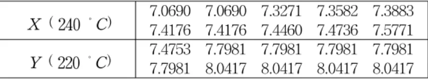
The data in Table 1 are taken from Nelson (1990) and represent the hours to failure of 20 motorettes with a new class-H insulation run at 240 ^∘C and 220^∘C. It has been observed by Nelson (1990) that lognormal distribution adequately fits at the two temperatures. Note that X and Y denote the nature logarithm of the failure times in the Table 1. We thus assume that the below data come from independent normal distributions.

Table 1: Failure Times at the Two Temperatures X ( 240^∘C) 7.0690 7.0690 7.3271 7.3582 7.3883

7.4176 7.4176 7.4460 7.4736 7.5771 Y ( 220^∘C) 7.4753 7.7981 7.7981 7.7981 7.7981 7.7981 8.0417 8.0417 8.0417 8.0417

For the equality of the CV, the score test developed by Gupta and Ma (1996).

That is, under H₁, the test statistics is given by Z = ˆγ²(1+2 γˆ²)

2 ( a²₁

n₁ + a²₂ n₂ ), where

a₁= ∑

n1

i= 1

(x_i- μˆ

1)² ˆμ

1

2 ˆγ³ - n₁

ˆ , aγ ²= ∑

n2

i= 1

(y_i- μˆ

2)² ˆμ

2

2 ˆγ³ - n₂ ˆγ

and μˆ_{1, μ}ˆ_{2, γ}ˆ is maximum likelihood estimator of μ₁,μ₂,γ. Under H₁, Z has a chi-square distribution with 1 degree of freedom. Since ˆμ

1= 7.354238, ˆμ

2= 7.863381 and γˆ = 0.021644, the observed value of the test statistic Z is 0.0113. Hence H₁ not rejected and the p-value of the test is almost one (Gupta, Ramakrishnan and Zhou, 1999).

The value of fractional Bayes factor of H2 versus H1 is B^F₂₁= 0.2939. We assume that the prior probabilities are equal. Then the posterior probability for H1

is 0.7729. Thus there are strong evidence for H1 in terms of the posterior probability.

Therefore both of the classical method and Bayes factor give reasonable answers in this example.

APPENDIX 1. Propriety of Posterior Distribution

Under the reference prior π(μ,γ)=μ ^{- 1}γ^{- 1}(1+2γ²)^{- 1/2}, the joint posterior for μ,γ given x is

π( μ,γ∣ x )∝μ^{- ( n + 1)}γ^{- ( n + 1)}(1+2γ²)^{- 1/2}exp { - ∑

n

i = 1(x_i-μ)² 2γ²μ² }.

Since (1+2γ²)^{- 1/2}≤2^{- 1/2}γ^{- 1}, thus

π(μ,γ∣ x)≤C₁μ^{- ( n + 1)}γ^{- ( n + 2)}exp { -

∑ⁿ

i = 1(x_i-μ)²

2γ²μ² }, (3) where C₁ is a constant. Integrating with respect to γ in (3), then

C₂[∑

n

i = 1(x_i-μ)²]^-

n + 1

2 = C₃[1+ n( x- μ)² S² ]^-

n + 1 2 ,

where S²= ∑ⁿ

i = 1(x_i- x)² and C2 and C3 are a constant. Thus the above form has a Student- t with n degrees of freedom. Thus the posterior distribution is proper. This completes the proof. □

REFERENCES

1. Berger, J. O. and Bernardo, J. M. (1989). Estimating a Product of Means : Bayesian Analysis with Reference Priors. Journal of the American Statistical Association, 84, 200-207.

2. Berger, J. O. and Bernardo, J. M. (1992). On the Development of Reference Priors (with discussion). Bayesian Statistics IV, J. M.

Bernardo, et. al., Oxford University Press, Oxford, 35-60.

3. Berger, J. O. and Pericchi, L. R. (1996). The Intrinsic Bayes Factor for Model Selection and Prediction, Journal of the American Statistical Association, 91, 109-122.

4. Doornbos, R. and Dijkstra, J. B. (1983). A Multi Sample Test for the Equality of Coefficients of Variation in Normal Populations.

Communication in Statistics-Simulation and Computation, 12, 147-158.

5. Jeffreys, H. (1961). Theory of Probability. Oxford University Press, New York.

6. Lohrding, R. K. (1969). A Test of Equality of Two Normal Means

Assuming Homogeneous Coefficients of Variation. The Annals of Mathematical Statistics, 40, 1374-1385.

7. Gupta, R. C. and Ma, S. (1996). Testing the Equality of Coefficient of Variation in k Normal Populations. Communication in Statistics-Theory and Methods, 25, 115-132.

8. Gupta, R. C., Ramakrishnan, S. and Zhou, X. (1999). Point and Interval Estimation of P( X< Y) : The Normal Case with Common Coefficient of Variation. Annals of the Institute of Statistical Mathematics, 51, 571-584.

9. Lee, H. C. and Kang, S. G. (2003). Reference Priors in the Normal Distributions with Common Coefficient of Variation. Journal of Korean Data & Information Science Society, 14, 697-705.

10. Miller, E. C. and Karson, M. J. (1977). Testing Equality of Two Coefficients of Variation. American Statistical Association: Proceedings of the Business and Economics Section, Part I, 278-283.

11. Nelson, W. (1990). Accelerated Testing, Wiley, New York.

12. O' Hagan, A. (1995). Fractional Bayes Factors for Model Comparison (with discussion), Journal of Royal Statistical Society, B, 57, 99-118.

13. Sinha, B. K., Rao, B. R. and Clement, B. (1978). Behrens-Fisher Problem under the Assumption of Homogeneous Coefficients of

Variation. Communication in Statistics-Theory and Methods, 7, 637-656.

14. Rao, K. A. and Vidya, R. (1992). On the Performance of a Test for Coefficient of Variation. Calcutta Statistical Association Bulletin, 42, March and June, 165-166, 87-95.

15. Spiegelhalter, D. J. and Smith, A. F. M. (1982). Bayes Factors for Linear and Log-Linear Models with Vague Prior Information, Journal of Royal Statistical Society, B, 44, 377-387.

[ received date : Sep. 2003, accepted date : Nov. 2003 ]