The Admissible Multiperiod Mean Variance
Portfolio Selection Problem
with Cardinality Constraints
Peng Zhang*, Bing Li
School of Management, Wuhan University of Science and Technology, Wuhan, China (Received: May 9, 2016 / Accepted: November 4, 2016)
ABSTRACT
Uncertain factors in finical markets make the prediction of future returns and risk of asset much difficult. In this paper, a model,assuming the admissible errors on expected returns and risks of assets, assisted in the multiperiod mean va-riance portfolio selection problem is built. The model considers transaction costs, upper bound on borrowing risk-free asset constraints, cardinality constraints and threshold constraints. Cardinality constraints limit the number of assets to be held in an efficient portfolio. At the same time, threshold constraints limit the amount of capital to be invested in each stock and prevent very small investments in any stock. Because of these limitations, the proposed model is a mix integer dynamic optimization problem with path dependence. The forward dynamic programming method is designed to obtain the optimal portfolio strategy. Finally, to evaluate the model, our result of a meaning example is compared to the terminal wealth under different constraints.
Keywords: Multiperiod Portfolio Selection, Admissible Return, Admissible Variance, Cardinality Constraints Constraints, The Forward Dynamic Programming Method
* Corresponding Author, E-mail: [email protected]
1. INTRODUCTION
The portfolio selection problem decides the choice of limited capital to a number of potential assets accord-ing to a profitable investment strategy. The pioneeraccord-ing work of the portfolio selection problem is the concept of efficient set developed by Markowitz (1952). In his se-minal work based on modern portfolio theory, Markowitz viewed portfolio selection as a mean-variance optimiza-tion problem with regard to two criteria: to maximize the expected return of a portfolio, and to minimize the va-riance of return. More formally, a desirable portfolio is defined to be a tradeoff between risk and expected return. It combines probability theory with optimization tech-niques to model the investment behavior under
uncertain-ty. Mean variance model makes a basic assumption that the trend of asset markets in future can be simulated by current and before asset data. The mean and covariance are the most important indicators in portfolio selection problem; thus, the assumption means that is, the mean and covariance of assets in future is similar to the past one. Although we have to say that it is very hard to ensure the assumption is always correct in the real ever-changing asset markets, the assumption is much common in lots of works about this problem (see Yu et al., 2010).
The portfolio selection model based on fuzzy proba-bilities has proposed by Tanaka et al. (2000). The mean vector and covariance matrix in the model designed by Markowitz are respectively replaced by the fuzzy weighted average vector and covariance matrix. It can be regarded Vol 16, No 1, March 2017, pp.118-128 https://doi.org/10.7232/iems.2017.16.1.118
as a natural extension of the model given by Markowitz because of the close relationship between probability theory and fuzzy probability. Its approach permits the incorporation of expert knowledge by means of a possi-bility grade, to reflect the similarity between the future state of asset markets and the state of previous periods. By using fuzzy approaches, the knowledge of the experts and the subjective opinions of the investors can be better integrated into a portfolio selection model. Zhang and Nie (2004), Zhang et al. (2006), and Zhang and Wang (2008) discussed the admissible efficient portfolio selection us-ing the assumption that the expected return and risk of assets have admissible errors to reflect the uncertainty in real investment actions. Then, an analytic derivation of admissible efficient frontier is given, when short sales were not allowed on all risky assets. Dubois and Prade (1988) defined an interval-valued expectation of fuzzy numbers which is set as consonant random sets. They also showed that this expectation remains additive in the sense of addition of fuzzy numbers. Carlsson and Fullér (2001) employed possibility distributions by introducing lower and upper possibilistic mean values of fuzzy numbers. Huang (2008) proposed mean risk curve portfolio selec-tion models. Li et al. (2010) proposed mean- variance-skewness fuzzy portfolio which can be solved bya genet-ic algorithm and fuzzy simulation. Carlsson et al. (2002) introduced a possibilistic approach to select portfolios with highest utility score under the assumption that the returns of assets are trapezoidal fuzzy numbers.
Many modifications are proposed to improve the ac-curacy of the Markowitz’s mean variance portfolio selec-tion model, for example, limiting the number of assets to be held in an efficient portfolio (cardinality constraints) or prescribes lower and upper bounds on the fraction of the capital invested in each asset (threshold constraints). These improvements are based on real-world practices; however, it is clearly not desirable to administer a portfo-lio made up of a large number of assets because of trans-action costs, complexity of management, or the policies of asset management companies. The model (often called cardinality constrained Markowitz model), and its varia-tions have been fairly intensively studied in the last dec-ade. Some researchers proposed exact solution methods (ie., Bienstock, 1996; Bertsimas and Shioda, 2009; Li et
al., 2006; Shaw et al., 2008; Murray and Shek, 2012);
Cesarone et al., 2013; Cui et al., 2013; Sun et al., 2013; Le Thi et al., 2009, 2014). Since exact solution methods were able to solve only a fraction of practically useful LAM models, many heuristic algorithms had also been proposed (ie.,Fernández and Gómez, 2007; Ruiz-Torrubiano and Suarez, 2010; Anagnostopoulos and Mamanis, 2011; Woodside-Oriakhi et al., 2011; Deng et al., 2012). In these studies, it appears that the computational complexi-ty of the solution given by the LAM (Limited Asset Mar-kowitz) model is much greater than the one spent by the
classical Markowitz model. Indeed, the standard Marko-witz model is a convex quadratic programming problem, while the LAM model is a mixed integer quadratic pro-gramming problem which is a NP-hard problem. Clearly, the computational complex of LAM model is much im-proved.
Although the case of a long-term investment is of greater importance in practice, much less has been done in that area. Although it is heavily discussed in the recent literatures (see e.g., Li and Ng, 2000; Zhu et al., 2004; Brandt et al., 2006; Gülpınar and Rustem, 2007; Çeli-kyurt and Özekici, 2007; Calafiore, 2008; Yan et al., 2009, 2012; Yu et al., 2010, 2012; Wu and Li, 2012; Li and Li, 2012; Zhang et al., 2012, 2014; Liu et al., 2012, 2013; Zhang and Zhang, 2014; Bodnar et al., 2015). To the best of our knowledge, a closed-form solution is not available in the general case up to now. Closed-form solu-tions are only presented with the assumption of indepen-dence by Li and Ng (2000), Zhu et al. (2004), Yan et al. (2009, 2012), Yu et al. (2010, 2012), Wu and Li (2012), Li and Li (2012). For more general models, the solution is frequently determined by a numerical procedure (see e.g., van Binsbergen and Brandt, 2007; Mansini et al., 2007; Gülpınar and Rustem, 2007; Zhang et al., 2012, 2014; Liu
et al., 2012, 2013; Zhang and Zhang, 2014; Köksalan and
Şakar, 2014).
Since the return of asset is in a fuzzy uncertain eco-nomic environment and varies all the time, its expected return and risk cannot accurately be predicted. Based on this fact, it is reasonable to assume that the expected re-turn and risk have admissible errors. This paper deals with the portfolio selection problem based on this as-sumption that the expected return and risk of asset have admissible errors to show the uncertainty in real invest-ments. The contribution of this work is as follows. We propose a new admissible multiperiod mean variance portfolio selection with upper bound on borrowing risk-free asset constraints, transaction costs, threshold con-straints and cardinality concon-straints. Cardinality concon-straints limit the number of assets held in an efficient portfolio. Threshold constraints limit the amount of capital to be invested in each stock; moreover, very small investments in any stock are prevented according to its strategy. Then, a novel forward dynamic programming method is em-ployed to find the solution. Finally, we give an important example to illustrate the idea of the model. More impor-tantly, the results compared to other methods of the ex-ample demonstrate the effectiveness of the designed algo-rithm.
This paper is organized as follows. In Section 2, we present the admissible efficient multiperiod portfolio model and define the upper and lower admissible efficient mul-tiperiod portfolio frontiers by the spreads of the portfolio expected returns and risks from the upper and lower bounds of admissible errors. Transaction costs, upper
bound on borrowing constraints, the threshold constraints and cardinality constraints are formulated into the multi-period portfolio. A new admissible multimulti-period portfolio selection model is constructed. A forward dynamic pro-gramming method is proposed to solve it in Section 3. In Section 4, A numerical example is given to illustrate our proposed effective means and approaches, and the ter-minal wealth under different constraints are compared in Section 4, Finally, some conclusions are given in Section 5.
2. THE ADMISSIBLE MULTIPERIOD PORTFOLIO SELECTION MODEL
In this paper, we take a very interest assumption that there are n risky assets and one risk-free asset in the fi-nancial market. An investor allocates his initial wealth W1 among n +1 assets at the beginning of time period 1, and obtains the terminal wealth at the end of time period T. The total process of this investment last from the begin-ning of period 1 to the end of period T. The investor can modification the choice of the n risky assets at the begin-ning of each period during the process of investment. Suppose that the returns of portfolios among different periods are independent of each other. In order to describe conveniently, we use the following notations:
it
x the investment proportion of risky asset i at pe-riod t;
xi0 the initial investment proportion of risky asset i at period 1;
xt the portfolio at period t, where xt = (x1t, x2t , ... , xnt)’;
xft the investment proportion of risk-free asset at period t, where 1 1 n ft it i x x = = −
∑
; xbft upper bound on borrowing risk-free asset at pe-riod t, where xft ≥ xbft, xbft ≤ 0;
Rit the random return of risky asset i at period t;
rit the expected return of Rit, where rt = (r1t, r2t , ..., rnt)’; σijt the covariance of Rit and Rjt;
rpt the expected return rate of the portfolio xt at pe-riod t;
rNt the net return rate of the portfolio xt at period t;
uit the upper bound constraints of xit;
lit the lower bound constraints of xit;
Wt the holding wealth at the beginning of period t;
rft the borrowing/lending rate of the risk-free asset at period t;
rbt the borrowing rate of the risk-free asset at pe-riod t;
rlt the lending rate of the risk-free asset at period t;
cit the unit transaction cost of risky asset i at period
t;
K the desired number of assets in the portfolio at
period t.
where prime (’) denotes matrix transposition and all non-primed vectors are column vectors.
Let the borrowing rate of the risk-free asset at pe-riod t be larger than the lending rate of the risk- free asset, ie. rbt ≥ rlt. If the borrowing is allowed on the risk free asset, then the expected return associated with portfolio xt are given as follows:
1 1 (1 ), 1, , n n pt it it ft it i i r r x r x t T = = =
∑
+ −∑
= " (1) where 1 1 , 1 0 , 1 0 n lt it i ft n bt it i r x r r x = = ⎧ − ≥ ⎪⎪ = ⎨ ⎪ − ≤ ⎪⎩∑
∑
. 1 1 n it 0 i x = −∑
≥ ,means that lending of the risk-free asset is allowed; otherwise , it represents the borrowing from the risk-free asset .
The variance of the portfolio xt can be expressed as
1 1 ( ) n n t t t it ij jt i j V x xσ x = = =
∑∑
(2)Since the economic environment is uncertain and rit,
I = 1, ... , n varies in the process of investment, the future
states of n risky assets returns cannot be predicted accu-rately. We extend the admissible average returns and co-variances of singleperiod portfolio selection in Zhang and Nie (2004), Zhang et al. (2006), and Zhang and Wang (2008) to multiperiod portfolio selection. Thus, the ad-missible average returns and covariances at period t are, respectively, defined as , , 1, , , 1, , t t t t it it i il i ih r = +r φ φ ≤φ ≤φ i= " n t= " T (3) and , , 1, , , 1, , t t t t t t ij ij ij ijl ij ijh i n t T σ =σ +ε ε ≤ε ≤ε = " = " (4)
where φit denotes the admissible error for rit; φilt expresses the lower bound of φit; φiht is the upper bound of φit; εijt defines the admissible error for σijt; εijlt indicates the lower bound of εijt;εijht shows the upper bound of εijt. φilt, φiht, εijlt and εijht can be estimated by combining the forecasted information of the assets return with the opinion of ex-perts opinion. Correspondingly, the intervals [rit+φilt,
rit+φiht] and [σijt+εijlt, σijt+εijht] are determined. φit and εijt can be selected by an investor based on his attitude to return and risk.
The admissible average return vector can be defined by , , 1, , t t t t t t l h r = +r φ φ ≤φ ≤φ t= " T (5) where rt=(r1t, r2t, …, rnt)’, φt = (φ1t, φ2t, …, φnt)’,φlt = (φ1lt, φ2lt, …, φnlt)’, and φht=(φ1ht, φ2ht, …, φnh)’.
Similarly, the admissible covariance matrix can be denoted by , , 1, , t t t t t t l h V = +V ε ε ≤ε ≤ε t= " T (6) where Vt=( ) , ( ) , 1 ( )1 t t t t t ij n n ij n n ij n n s × e = e × e = e × and ( ) t t h ijh n n e = e ×
The admissible expected value and variance of the return associated with portfolio xt are respectively given by ' ' ( t) (1 ), 1, , pt t t ft t r = r+φ x +r −e x t= " T (7) and ' ( ) ( t) t t t t t V x =x V +ε x (8) where e = (1, 1, …, 1).
For any xt ≥ 0, it follows that ' ' ' ' ( t) (1 ) ( t) (1 ) t l t ft t pt t h t ft t r+φ x +r −e x ≤r ≤ r +φ x +r −e x and '( t) ( ) '( t) t t l t t t t t h t x V +ε x ≤V x ≤x V +ε x
We assume in the sequel that the transaction costs at period t is a V shape function of difference between the
tth period portfolio xt = (x1t, x2t , ", xnt) and the t−1 th period portfolio xt−1 = (x1t−1 ,x2t−1 , ", xnt−1). That’s to say, the transaction cost for asset i at period t can be expressed by
1
it it it it
C =c x −x− (9)
Hence, the total transaction costs of the portfolio xt = (x1t, x2t , . . . , xnt) at period t can be represented as
1 1 , 1, , n t it it it i C c x x− t T = =
∑
− = " (10)Thus, the admissible net return rate of the portfolio xt at period t can be denoted as
' ' 1 1 1 =1 1 1 ( ) (1 ) = ( ) (1 ) n t Nt t t ft t it it it i n n n t it i it ft it it it it i i i r r x r e x c x x r x r x c x x φ φ − = − = = = + + − − − + + − − −
∑
∑
∑
∑
(11)Then, the admissible holding wealth at the beginning of the period t can be written as
1 (1 ) t t Nt W+ =W +r =1 1 1 1 (1 ( ) (1 ) ), 1, , n n t t it i it ft it i i n it it it i W r x r x c x x t T φ = − = = + + + − − − =
∑
∑
∑
" (12)To formulate cardinality constraints into the multipe-riod portfolio model, zero-one decision variables are add-ed as:
1 if any of asset of period ( =1, , ; =1, , ) is held 0 otherwise i t zit i n t T ⎧ ⎪ ⎨ ⎪ ⎩ = " " (13) where 1 . n it i z K = ≤
∑
The threshold constraints of multiperiod portfolio se-lection can be expressed as
it it it
l ≤x ≤u (14)
where lit and uit are respectively the lower and upper bounds constraints of xit.
A rational investor wishes to not only maximize ad-missible net return but also minimize the adad-missible va-riance of the rate of return on a portfolio. Thus, it is very important to get a tradeoff of these two objectives. Let (1−θ) andθ be the preference coefficients associated with criteria rNt and V xt( )t respectively. Then the investor
attempts to maximize 1 =1 1 1 1 1 ( , ( )) (1 ) 1 ( ) (1 ) ( ) n n n t t Nt t t it i it ft it it it it i i i n n t t it ij ij jt i j F r V x r x r x c x x x x θ φ θ σ ε − = = = = ⎛ ⎞ = − ⎜+ + + − − − ⎟ ⎝ ⎠ ⎛ ⎞ − ⎜ + ⎟ ⎝ ⎠
∑
∑
∑
∑∑
(15)where φit denotes the admissible error for rit, εijt denotes the admissible error for σijt. Here the parameter θ can be interpreted as the risk aversion factor of a investor. The greater the factor w is, the more risk aversion the investor has. In this paper, we assume that the investor is of risk aversion, i.e., 0 ≤ θ ≤ 1.
Thus, we construct the following admissible multi-period portfolio selection model with cardinality
con-straints: 1 1 =1 1 1 1 1 max ((1 ) 1 ( ) (1 ) ( ) ) T n n n t it i it ft it it it it t i i i n n t t it ij ij jt i j r x r x c x x x x θ φ θ σ ε − = = = = = ⎛ ⎞ − ⎜ + + + − − − ⎟ ⎝ ⎠ ⎛ ⎞ − ⎜ + ⎟ ⎝ ⎠
∑
∑
∑
∑
∑∑
1 1 =1 1 1 1 (1 ( ) (1 ) ) (a) 1 (b) . , {0,1} n n n t t it i it ft it it it it t i i i n b it ft i it it W r x r x c x x W x x s t z K z φ + − = = = = + + + − − − − ≥ ≤ ∈∑
∑
∑
∑
1 (c) , 1, , , 1, , (d) n i it it it it it l z x u z i n t T = ⎧ ⎪ ⎪ ⎪ ⎪ ⎨ ⎪ ⎪ ⎪ ⎪ ≤ ≤ = = ⎩∑
" " (16)where constraint (a) denotes the wealth accumula-tion constraint; constraint (b) indicates the upper bound on borrowing risk-free asset constraints at period t; con-straint (c) represents the desired number of assets in the portfolio must not exceed the given value K; constraint (d) states threshold constraints of xit.
If (φt, εt) = (φ
ht, εlt), then (16) can be rewritten as: 1 1 =1 1 1 1 1 max ((1 ) 1 ( ) (1 ) ( ) ) T n n n t it ih it ft it it it it t i i i n n t t it ij ijl jt i j r x r x c x x x x θ φ θ σ ε − = = = = = ⎛ ⎞ − ⎜ + + + − − − ⎟ ⎝ ⎠ ⎛ ⎞ − ⎜ + ⎟ ⎝ ⎠
∑
∑
∑
∑
∑∑
1 1 =1 1 1 1 1 (1 ( ) (1 ) ) 1 . , {0,1} , 1, , , 1, , n n n t t it ih it ft it it it it t i i i n b it ft i n it it i it it it it it W r x r x c x x W x x s t z K z l z x u z i n t T φ + − = = = = ⎧ = + + + − − − ⎪ ⎪ ⎪ − ≥ ⎪ ⎨ ⎪ ⎪ ≤ ∈ ⎪ ⎪ ≤ ≤ = = ⎩∑
∑
∑
∑
∑
" " (17) If (φt, εt) = (φlt, εht), then (16) can be rewritten as:
1 1 =1 1 1 1 1 max ((1 ) 1 ( ) (1 ) ( ) ) T n n n t it il it ft it it it it t i i i n n t t it ij ijh jt i j r x r x c x x x x θ φ θ σ ε − = = = = = ⎛ ⎞ − ⎜ + + + − − − ⎟ ⎝ ⎠ ⎛ ⎞ − ⎜ + ⎟ ⎝ ⎠
∑
∑
∑
∑
∑∑
1 1 =1 1 1 1 1 (1 ( ) (1 ) ) 1 . , {0,1} , 1, , , 1, , n n n t t it il it ft it it it it t i i i n b it ft i n it it i it it it it it W r x r x c x x W x x s t z K z l z x u z i n t T φ + − = = = = ⎧ = + + + − − − ⎪ ⎪ ⎪ − ≥ ⎪ ⎨ ⎪ ⎪ ≤ ∈ ⎪ ⎪ ≤ ≤ = = ⎩∑
∑
∑
∑
∑
" " (18)The Model (17) means that the investor optimistical-ly estimates the return and risk. The Model (18) means that the investor pessimistically estimates the return and risk. The Model (16) covers the scenario when the inves-tor makes his portfolio selection neither too optimistically nor too pessimistically.
Definition 1. The optimal solution of (16), xt (rt +φt,
σt +εt) is called an admissible efficient portfolio. The op-timal solution of (17), xt (rt +φht, σt +εlt) is called an upper admissible efficient portfolio. The optimal solution of (18), xt (rt +φlt, σt +εht) is called a lower admissible effi-cient portfolio.
For each admissible error couple (φt, εt) given by the investor, an admissible efficient frontier can be obtained by (16). If φt = 0 and εt = 0, then the admissible efficient frontier is the classical efficient frontier. It is obvious that the admissible portfolio selection model shown in (16) is an extensions of the conventional multiperiod portfolio selection models.
3. SOLUTION ALGORITHM
In this section we formulate a numerical solution to (16) based on an essential assumptions. Our results about (16) will require the following assumptions to be satisfied.
Assumption 1. (i) rt +φt≠kl, for any k ∈R, (ii) σt +εt is a
semi-positive definite matrix.
Assumption 1 (i) is essential. Assumption 1 (ii) is easi-ly satisfied by a proper selection of εt.
Letyit= xit−xi t( 1)− . Then the Model (16) can be
turned into as follows.
1 =1 1 1 1 1 max ((1 ) 1 ( ) (1 ) ( ) ) T n n n t it i it ft it it it t i i i n n t t it ij ij jt i j r x r x c y x x θ φ θ σ ε = = = = = ⎛ ⎞ − ⎜ + + + − − ⎟ ⎝ ⎠ ⎛ ⎞ − ⎜ + ⎟ ⎝ ⎠
∑
∑
∑
∑
∑∑
1 =1 1 1 1 ( 1) ( 1) 1 (1 ( ) (1 ) ) 1 y . y ( ) , {0,1} , 1, , , 1, , n n n t t it i it ft it it it t i i i n b it ft i it it i t it it i t n it it i it it it it it W r x r x c y W x x x x s t x x z K z l z x u z i n t T φ + = = = − − = ⎧ = + + + − − ⎪ ⎪ ⎪ − ≥ ⎪ ⎪ ⎪ ≥ − ⎨ ⎪ ≥ − − ⎪ ⎪ ≤ ∈ ⎪ ⎪ ⎪ ≤ ≤ = = ⎩∑
∑
∑
∑
∑
" " (19)where the Model (19) is the admissible multiperiod portfolio selection.
In this section, the forward dynamic programming method is proposed to solve the Model (19).
The sub-problem of period t of the Model (19) can be transformed into =1 1 1 1 1 max(1 ) 1 ( ) (1 ) ( ) n n n t it i it ft it it it i i i n n t t it ij ij jt i j r x r x c y x x θ φ θ σ ε = = = = ⎛ ⎞ − ⎜ + + + − − ⎟ ⎝ ⎠ ⎛ ⎞ − ⎜ + ⎟ ⎝ ⎠
∑
∑
∑
∑∑
1 =1 1 1 1 ( 1) ( 1) 1 (1 ( ) (1 ) ) 1 y . y ( ) , {0,1} , 1, , n n n t t it i it ft it it it t i i i n b it ft i it it i t it it i t n it it i it it it it it W r x r x c y W x x x x s t x x z K z l z x u z i n φ + = = = − − = ⎧ = + + + − − ⎪ ⎪ ⎪ − ≥ ⎪ ⎪ ⎪ ≥ − ⎨ ⎪ ≥ − − ⎪ ⎪ ≤ ∈ ⎪ ⎪ ⎪ ≤ ≤ = ⎩
∑
∑
∑
∑
∑
" (20)In the following section, we provide the detailed procedure of the forward dynamic programming method for finding optimal solutions of the Model (19). The pro-cedure of the algorithm can be showed as follows:
Algorithm The forward dynamic programming
me-thod:
Step1. When t = 1, W1 and x0 = (x10, …, xn0)’ have been given, the sub-problem of period 1 of the Model (19) can be transformed into 1 1 1 1 1 1 1 =1 1 1 1 1 1 1 1 1 max(1 ) 1 ( ) (1 ) ( ) n n n i i i f i i i i i i n n i ij ij j i j r x r x c y x x θ φ θ σ ε = = = = ⎛ ⎞ − ⎜ + + + − − ⎟ ⎝ ⎠ ⎛ ⎞ − ⎜ + ⎟ ⎝ ⎠
∑
∑
∑
∑∑
1 2 1 1 1 1 1 1 1 =1 1 1 1 1 1 1 1 0 1 1 0 1 1 1 1 1 1 1 1 (1 ( ) (1 ) ) 1 y . y ( ) , {0,1} , 1, , n n n i i i f i i i i i i n b i f i i i i i i i n i i i i i i i i W r x r x c y W x x x x s t x x z K z l z x u z i n φ = = = = ⎧ = + + + − − ⎪ ⎪ ⎪ − ≥ ⎪ ⎪⎪ ≥ − ⎨ ⎪ ≥ − − ⎪ ⎪ ≤ ∈ ⎪ ⎪ ⎪ ≤ ≤ = ⎩∑
∑
∑
∑
∑
" (21)If the matrix (σij1 + εij1)n×n is a semi-positive definite matrix, the Model (21) is a cardinality constrained convex quadratic programming problem. The optimal solution of the Model (21), * * * '
1 ( ,11 , n1)
x = x " x can be obtained by
branch-and-bound implementation with pivoting algo-rithms (Bertsimas and Shioda, 2009). At the same time,
1 * * * 1 1 1 1 1 1 =1 1 1 * 1 1 * 1 1 1 1 (1 ) 1 ( ) (1 ) ( ) n n n i i i f i i i i i i n n i ij ij j i j r x r x c y x x θ φ θ σ ε = = = = ⎛ ⎞ − ⎜ + + + − − ⎟ ⎝ ⎠ ⎛ ⎞ − ⎜ + ⎟ ⎝ ⎠
∑
∑
∑
∑∑
and * 2W can be obtained, respectively.
Step2. When t = m (m≥1 and m∈Z+), * 1 m W + and * * * ' 1 ( , , ) m m nm
x = x " x have been obtained, the sub-problem of
period m of the Model (19) can be transformed into
1 ( 1) ( 1) 1 ( 1) ( 1) ( 1) =1 1 1 ( 1) ( 1) ( 1) ( 1) 1 1 max(1 ) 1 ( ) (1 ) ( ) n n n i m i i m f i m i m i m i i i n n m m i m ij ij j m i j r x r x c y x x θ φ θ σ ε + + + + + = = + + + + = = ⎛ ⎞ − ⎜ + + + − − ⎟ ⎝ ⎠ ⎛ ⎞ − ⎜ + ⎟ ⎝ ⎠
∑
∑
∑
∑∑
( 1) * ( 2) ( 1) ( 1) ( 1) ( 1) ( 1) ( 1) ( 1) =1 1 1 ( 1) ( 1) 1 * ( 1) ( 1) * ( 1) ( 1) ( 1) ( 1) 1 ( 1) ( (1 ( ) (1 ) ) 1 y . y ( ) , {0,1} n n n m m i m i i m f m i m i m i m m i i i n b i m f m i i m i m im i m i m im n i m i m i i m i m W r x r x c y W x x x x st x x z K z l z φ + + + + + + + + + = = + + = + + + + + + = + + = + + + − − − ≥ ≥ − ≥− − ≤ ∈ ∑ ∑ ∑ ∑ ∑ 1) xi m( 1)+ ui m(+1) ( 1)zi m+,i 1, ,n ⎧ ⎪ ⎪ ⎪ ⎪ ⎪ ⎪ ⎨ ⎪ ⎪ ⎪ ⎪ ⎪ ⎪ ≤ ≤ = ⎩ " (22)If the matrix (σij(m+1)+εij(m+1))n×n is a semi-positive de-finite matrix, the Model (22) is a cardinality constrained convex quadratic programming problem. The optimal solution of the Model (22), * * * '
1 ( 1, , 1)
m m nm
x + = x + " x + can be
obtained by branch-and-bound implementation with pi-voting algorithms (Bertsimas and Shioda, 2009). At the same time, 1 * * * ( 1) ( 1) 1 ( 1) ( 1) ( 1) =1 1 1 * ( 1) ( 1) * ( 1) ( 1) 1 1 (1 ) 1 ( ) (1 ) ( ) n n n i m i i m f i m i m i m i i i n n m m i m ij ij j m i j r x r x c y x x θ φ θ σ ε + + + + + = = + + + + = = ⎛ ⎞ − ⎜ + + + − − ⎟ ⎝ ⎠ ⎛ ⎞ − ⎜ + ⎟ ⎝ ⎠
∑
∑
∑
∑∑
and * 2 mW + can be obtained, respectively.
Step3. If t = T, then the maximization of the terminal utility * * * =1 1 1 (1 ) 1 n ( T) (1 n ) n iT i iT fT iT iT iT i i i r x r x c y θ φ = = ⎛ ⎞ − ⎜ + + + − − ⎟ ⎝
∑
∑
∑
⎠ * * 1 1 ( ) n n T T iT ij ij jT i j x x θ σ ε = = ⎛ ⎞ − ⎜ + ⎟ ⎝∑∑
⎠ and * 1 T W+ can be obtained,respectively. Otherwise t = m+1, then turn Step 2. At period t, the global optimal solutions of the Model (21) and Model (22), which are the sub-problem of the Model (19) . can be obtained by branch-and-bound im-plementation with pivoting algorithm (Bertsimas and Shioda (2009)). So the global optimal solution of the Model (19) can also be known by the forward dynamic programming method. As a result, the global optimal so-lution of Model (16) can also be obtained.
The optimal solutions of (17) can be obtained as (φt, εt) = (φht, εlt). The optimal solutions of (18) can be obtained as (φt, εt) = (φ
lt, εht). Correspondingly, both the upper and lower admissible optimal solutions can also be indicated by the forward dynamic programming method.
4. NUMERICAL EXAMPLE
In this section, a numerical example is given to ex-press the idea of the proposed model. Assume that an investor chooses twenty stocks from Shanghai Stock Ex-change for his investment. The stocks codes are respec-tively S1 (600036), S2 (600002), S3 (600060), S4 (600362),
S5 (600519), S6 (601111), S7 (601318), S8 (600900), S9 (600887), S10 (600690), S11 (6000970), S12 (600000), S13 (600009), S14 (600019), S15 (600029), S16 (600104), S17 (600315), S18 (600518), S19 (600570), S20 (600880). He intends to make five periods of investment with initial wealth W1 = 1 and his wealth can be adjusted at the be-ginning of each period. It is assumed that the returns, risk and turnover rates of the twenty stocks at each period are represented as trapezoidal fuzzy numbers. We collect historical data of them from April 2006 to March 2015 and set every three months as a period to handle the his-torical data.
The transaction costs of assets of the two periods take the same value cit = 0.003 (i = 1, …, 20; t = 1, …, 5), the desired number of assets in the portfolio K = 0, …, 9 at period t, t = 1, …, 5, upper bound on borrowing risk-free asset xb
ft = −0.5, preference coefficient θ = 0, 0.1,…1, the borrowing rate of the risk-free asset rbt = 0.017, the lending rate of the risk-free asset rlt = 0.009, t = 1, …, 5, the lower lit = 0.05 and upper bound constraints uit = 0.2 (i = 1, …, 20; t = 1, …, 5).
In this example, x0, φht, φlt and εijt are given by
x0 = (0, 0, 0, 0, 0, 0, 0, 0, 0, 0, 0, 0, 0, 0, 0, 0, 0, 0, 0, 0)’, φht = (0.025, 0.015, 0.01, 0.015, 0.025, 0.015, 0.045, 0.015, 0.045, 0.015, 0.025, 0.01, 0.01, 0.01, 0.01, 0.01, 0.01, 0.015, 0.01, 0.015)’, φlt = φht, εijt = 0, I = 1, …, 20, j = 1, …, 20.
By using the forward dynamic programming method to solve the Model (16), Model (17) and Model (18), the corresponding results can be obtained as follows.
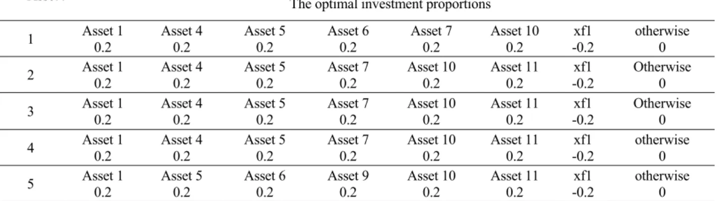
If φit = 0, εijt = 0, θ = 0.5, K = 6, the optimal solution of the admissible multiperiod portfolio selection (Model (16)) is shown in the Table 1.
When φit =0, εijt = 0, θ = 0.5, K = 6, the optimal in-vestment strategy at period 1 is x11 = 0.2, x41 = 0.2, x51 = 0.2, x61 = 0.2, x71 = 0.1, x101 = 0.2, xf1 = −0.2 and the rest of variables equal to zero, which means investor should allocate his initial wealth on asset 1, asset 4, asset 5, asset 6, asset 7 , asset 10, risk-free asset and otherwise assets by the proportions of 20%, 20%, 30%, 20%, 20% , 20%, −20% and the rest of variables equal to zero, respectively. In Table 1, the optimal investment strategies at period 2, period 3, period 4 and period 5 can also be obtained. In this case, the available terminal wealth is 1.9236.
If φit = 0, εijt = 0, θ = 0.5, K = 8, the optimal solution of Model (16) will be obtained as the Table 2. The availa-ble terminal wealth is 2.0611.
To display the influence of K on the optimal solution of multiperiod, its value is respectively set as 6 and 8, and the Model (16) for portfolio decision-making will be
Table 1. The optimal solution of Model (16) when φit = 0, εijt = 0, θ = 0.5, K = 6
Asset i
t The optimal investment proportions
1 Asset 1 0.2 Asset 4 0.2 Asset 5 0.2 Asset 6 0.2 Asset 7 0.2 Asset 10 0.2 -0.2 xf1 otherwise 0 2 Asset 1 0.2 Asset 4 0.2 Asset 5 0.2 Asset 7 0.2 Asset 10 0.2 Asset 11 0.2 -0.2 xf1 Otherwise 0 3 Asset 1 0.2 Asset 4 0.2 Asset 5 0.2 Asset 7 0.2 Asset 10 0.2 Asset 11 0.2 -0.2 xf1 Otherwise 0 4 Asset 1 0.2 Asset 4 0.2 Asset 5 0.2 Asset 7 0.2 Asset 10 0.2 Asset 11 0.2 -0.2 xf1 otherwise 0 5 Asset 1 0.2 Asset 5 0.2 Asset 6 0.2 Asset 9 0.2 Asset 10 0.2 Asset 11 0.2 -0.2 xf1 otherwise 0
Table 2. The optimal solution when φit = 0, εijt = 0, θ = 0.5, K = 8
Asset i
t The optimal investment proportions
1 Asset 1 0.2 Asset 2 0.2 Asset 4 0.2 Asset 5 0.2 Asset 6 0.2 Asset 7 0.2 Asset 10 0.2 Asset 11 0.1 −0.5 xf1 2 Asset 1 0.2 Asset 2 0.2 Asset 4 0.2 Asset 5 0.2 Asset 6 0.1886 Asset 7 0.2 Asset 10 0.2 Asset 11 0.1114 −0.5 xf1 3 Asset 1 0.2 Asset 2 0.2 Asset 4 0.2 Asset 5 0.2 Asset 6 0.1 Asset 7 0.2 Asset 10 0.2 Asset 11 0.2 −0.5 xf1 4 Asset 1 0.2 Asset 4 0.2 Asset 5 0.2 Asset 6 0.1638 Asset 7 0.2 Asset 10 0.2 Asset 11 0.2 Asset 18 0.1362 xf1 −0.5 5 Asset 1 0.2 Asset 5 0.2 Asset 6 0.2 Asset 7 0.1861 Asset 9 0.2 Asset 100.2 Asset 11 0.2 Asset 18 0.1139 −0.5 xf1
used afterwards. After using forward dynamic program-ming method, the corresponding optimal investment strategies can be obtained as shown in Table 1 and Table 2. According to the results shown in Table 1 and Table 2, it can be seen that most of assets of the optimal solutions of K = 6 and K = 8 are the same. There are six assets of the same values in period 1, i.e. asset 1, asset 4, asset 5, asset 6, asset 7, asset 10.
If φht = (0.025, 0.015, 0.01, 0.015, 0.025, 0.015, 0.015, 0.015, 0.015, 0.015, 0.025, 0.01, 0.01, 0.01, 0.01, 0.01, 0.01, 0.015, 0.01, 0.015)’, ε
ijt = 0, θ = 0.5, K = 6, the optimal solution of he upper admissible multiperiod port-folio selection (Model (17)) will be obtained as the Table 3. When θ = 0.5, K = 6, the available terminal wealth is 2.0946. If φlt =-φht, εijt = 0, θ = 0.5, K = 6, the optimal solution of the lower admissible multiperiod portfolio selection (Model (18)) will be obtained as the Table 4. Its available terminal wealth is 1.8107.
Table 1, Table 3 and Table 4show thatwhenθ = 0.5,
K = 6, the optimal solutions of the Model (16), the Model
(17) and the Model (18) are not the same, and the availa-ble terminal wealthof the three models are different. The terminal wealth of the upper admissible multiperiod port-folio selection (Model (17)) is the largest, and the termin-al wetermin-alth of the lower admissible multiperiod portfolio selection (Model (18)) is the smallest.
When θ = 0.5, K = 0, 1, …, 9, the optimal terminal wealth of the Model (16), the Model (17) and the Model (18) can respectively be obtained as shown in Table 5. W6 is the terminal wealth of the admissible mutiperiod port-folio selection when φit = 0, εijt = 0. UW6 is the terminal wealth of the optimistically admissible mutiperiod portfo-lio selection (the Model (17)). LW6 is the terminal wealth of the pessimistically admissible mutiperiod portfolio selection (the Model (18)).
Where W6 is the terminal wealth of the admissible
Table 3. The optimal solution of Model (17) when θ = 0.5, K = 6
Asset i
t The optimal investment proportions
1 Asset 1 0.2 Asset 4 0.2 Asset 5 0.2 Asset 7 0.2 Asset 9 0.2 Asset 10 0.2 xf1
−0.2 otherwise 0 2 Asset 1 0.2 Asset 4 0.2 Asset 5 0.2 Asset 7 0.2 Asset 9 0.2 Asset 10 0.2 xf1 −0.2 Otherwise 0 3 Asset 1 0.2 Asset 5 0.2 Asset 7 0.2 Asset 9 0.2 Asset 10 0.2 Asset 11 0.2 xf1
−0.2 Otherwise 0 4 Asset 1 0.2 Asset 5 0.2 Asset 7 0.2 Asset 9 0.2 Asset 10 0.2 Asset 11 0.2 xf1 −0.2 otherwise 0 5 Asset 1 0.2 Asset 5 0.2 Asset 6 0.2 Asset 9 0.2 Asset 10 0.2 Asset 11 0.2 xf1
−0.2 otherwise 0
Table 4. The optimal solution of Model (18) when θ = 0.5, K = 6
Asset i
t The optimal investment proportions
1 Asset 1 0.2 Asset 2 0.2 Asset 4 0.2 Asset 5 0.2 Asset 6 0.2 Asset 10 0.2 xf1
−0.2 otherwise 0 2 Asset 1 0.2 Asset 2 0.2 Asset 4 0.2 Asset 5 0.2 Asset 6 0.2 Asset 10 0.2 xf1
−0.2 Otherwise 0 3 Asset 1 0.2 Asset 4 0.2 Asset 5 0.2 Asset 6 0.2 Asset 10 0.2 Asset 11 0.2 xf1
−0.2 Otherwise 0 4 Asset 1 0.2 Asset 4 0.2 Asset 5 0.2 Asset 6 0.2 Asset 10 0.2 Asset 11 0.2 xf1 −0.2 otherwise 0 5 Asset 1 0.2 Asset 5 0.2 Asset 6 0.2 Asset 9 0.2 Asset 10 0.2 Asset 11 0.2 xf1 −0.2 otherwise 0
Table 5. The optimal terminal wealth of the Model (16-18) when θ = 0.5, K = 1, …, 9
K 0 1 2 3 4 5 6 7 8 9
W6 1.0450 1.2431 1.4322 1.5908 1.7231 1.8279 1.9236 2.0157 2.0611 2.0611
UW6 1.0450 1.2698 1.4855 1.6675 1.8240 1.9652 2.0946 2.2160 2.2579 2.2579
mutiperiod portfolio selection which φit = 0, εijt = 0.
UW6 is the terminal wealth of the optimistically admissi-ble mutiperiod portfolio selection (the Model (17)). LW6 is the terminal wealth of the pessimistically admissible mutiperiod portfolio selection (the Model (18)).
In the used data sets, the same optimal solutions at K = 8 is suitable for K ≥ 9. The experiments in this paper cor-respond to the values of K is the interval [0, 9]. It can be seen that, elaborated in Table 5, the terminal wealth also becomes larger, when the preset the desired number of as-sets in the portfolio become larger, this reflects the influ-ence of the desired number of assets on portfolio selection.
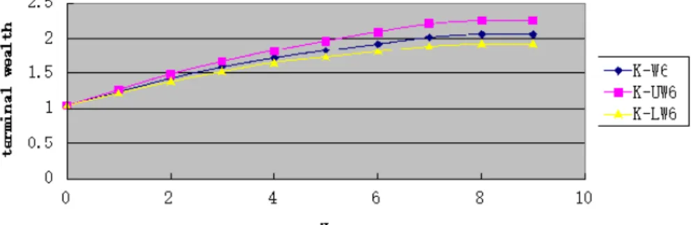
In order to address the relationship between the K and the terminal wealth of the Model (16), the Model (17) and the Model (18), Figure 1 based on the data in Table 5 is pointed as follow: K-W6 is the admissible terminal wealth of the Model (16) with different K; K-UW6 is the upper admissible terminal wealth of the Model (17) with different K; K-LW6 is the lower admissible terminal wealth of the Model (18) with different K,
In Figure 1, with the same value of Kthe terminal wealth of the upper admissible multiperiod portfolio se-lection is larger than the terminal wealth of the lower
ad-missible multipriod portfolio selection. For the terminal wealth under the conditions of φilt ≤ φit ≤ φiht and εijlt ≤ εijt ≤ εijht, the admissible multiperiod portfolio selection is at middle position between upper and lower admissible multiperiod portfolio selection.
When K = 8, θ = 0, 0.1, …, 0.9, 1, the optimal ter-minal wealth of the Model (16), the Model (17) and the Model (18) can be respectively obtained as shown in Ta-ble 6. W6 is the terminal wealth of the admissible mutipe-riod portfolio selection which φit = 0, εijt = 0. UW6 is the terminal wealth of the upper admissible mutiperiod port-folio selection (the Model (17)). LW6 is the terminal wealth of the lower admissible mutiperiod portfolio selec-tion (the Model (18)).
where W6 is the terminal wealth of the admissible mutiperiod portfolio selection which φit = 0, εijt = 0. UW6 is the terminal wealth of the upper admissible mutiperiod portfolio selection (the Model (17)). LW6 is the terminal wealth of the lower admissible mutiperiod portfolio selec-tion (the Model (18)).
From Table 6, the Figure 2, which reflect the relation-ship between the preference coefficients θ and the termin-al wetermin-alth of the Model (16), the Model (17) and the
Mod-Figure 1. The relationship between the K and the terminal wealth of the Model (16-18).
Table 6. The optimal terminal wealth of the Model (16-18) when K = 8, θ = 0, 0.1, …, 0.9, 1
θ 0 0.1 0.2 0.3 0.4 0.5 0.6 0.7 0.8 0.9 1
W6 2.0776 2.0771 2.0757 2.0732 2.0680 2.0611 2.0537 2.0396 2.0132 1.9498 1.0450
UW6 2.2843 2.2843 2.2843 2.2838 2.2773 2.2579 2.2652 2.2495 2.2202 2.1371 1.0450
LW6 1.9398 1.9398 1.9373 1.9351 1.9335 1.9261 1.9139 1.8961 1.8657 1.7972 1.0450
el (18), can be obtained as follows. PC is preference coef-ficients; PC-W6 is the admissible terminal wealth of the Model (16) with different θ; PC-UW6 is the upper admiss-ible terminal wealth of the Model (17) with different θ ; PC-LW6 is the lower admissible terminal wealth of the Model (18) with different θ .
In Figure 2, it can be seen that, if the θ has the same value same, the terminal wealth of the upper admissible multiperiod portfolio selection is above the terminal wealth of the lower admissible multipriod portfolio selec-tion. For φilt ≤ φit ≤φiht, εijlt ≤ εijt ≤εijht, the terminal wealth of the admissible multiperiod portfolio selection is the mid-dle of the terminal wealth of upper and lower admissible multiperiod portfolio selection. The terminal wealth be-comes smaller, when preference coefficient θ become larger, which gives the influence of preference coefficient θ on portfolio selection.
5. CONCLUSIONS
In this paper, we have discussed the admissible multi-period portfolio selection problem with transaction cost, borrowing constraints, threshold constraints and cardinali-ty constraints. In the proposed model, the cardinalicardinali-ty con-straints are used to control the number of assets held in an efficient portfolio. Because of the transaction cost and cardinality constraints, the multiperiod portfolio selection is a mix integer dynamic optimization problem with path dependence. The forward dynamic programming method is designed to obtain the optimal portfolio strategy. Final-ly, an example using real data from the Shanghai Stock Exchange is given to illustrate the behavior of the pro-posed model and the designed algorithm.
ACKNOWLEDGMENTS
This research was supported by the National Natural Science Foundation of China (no. 71271161).
REFERENCES
Anagnostopoulos, K. P. and Mamanis, G. (2011), The mean-variance cardinality constrained portfolio op-timization problem: An experimental evaluation of five multiobjective evolutionary algorithms, Expert
Systems with Applications, 38, 14208-14217.
Bertsimas, D. and Shioda, R. (2009), Algorithms for car-dinality-constrained quadratic optimization,
Compu-tational Optimization and Applications, 43, 1-22.
Bienstock, D. (1996), Computational study of a family of mixed-integer quadratic programming problems,
Mathe-matical Programming, 74, 121-140.
Bodnar, T., Parolya, N. and Schmid, W. (2015), A closed-form solution of the multi-period portfolio choice problem for a quadratic utility function, Annals of
Operations Research, 229(1), 121- 158.
Brandt, M. and Santa-Clara, P. (2006), Dynamic portfolio selection by augmenting the asset space, The Journal
of Finance, 61, 2187-2217.
Calafiore, G. C. (2008), Multi-period portfolio optimiza-tion with linear control policies, Automatica, 44(10), 2463-2473.
Carlsson, C. and Fullér, R. (2001), On possibilistic mean value and variance of fuzzy numbers, Fuzzy Sets and
Systems, 122, 315-326.
Carlsson, C., Fullér, R. and Majlender, P. (2002), A pos-sibilistic approach to selecting portfolios with high-est utility score, Fuzzy Sets and Systems, 131, 13-21. Cesarone, F., Scozzari, A. and Tardella, F. (2013), A new
method for mean-variance portfolio optimization with cardinality constraints, Annals of Operations
Research, 205, 213-234.
Cui, X. T., Zheng, X. J., Zhu, S. S., and Sun, X. L. (2013), Convex relaxations and MIQCQP reformulations for a class of cardinality-constrained portfolio selection problems, Journal of Global Optimization, 56, 1409-1423.
Çlikyurt, U. and Öekici, S. (2007), Multiperiod portfolio optimization models in stochastic markets using the mean-variance approach, European Journal of
Op-erational Research, 179(1), 186-202.
Deng, G. F., Lin, W. T., and Lo, C. C. (2012), Marko-witz-based portfolio selection with cardinality con-straints using improved particle swarm optimization,
Expert Systems with Applications, 39, 4558-4566.
Dubois, D. and Prade, H. (1988), Possibility Theory, Ple-num Perss, New York.
Fernández, A. and Gómez, S. (2007), Portfolio selection using neural networks, Computers & Operations
Re-search, 34, 1177-1191.
Gülpınar, N. and Rustem, B. (2007), Worst-case robust decisions for multi-period mean-variance portfolio optimization, European Journal of Operational
Re-search, 183(3), 981-1000.
Huang, X. (2008), Risk Curve and Fuzzy Portfolio Selec-tion, Computers and Mathematics with Applications,
55, 1102-1112.
Köksalan, M. and Şakar, C. T. (2014), An interactive approach to stochastic programming-based portfolio optimization, To Appear in Annals of Operations
Re-search.
Le Thi, H. A., Moeini, M., and Dinh, T. P. (2009), Portfo-lio selection under downside risk measures and car-dinality constraints based on DC programming and DCA, Computational Management Science, 6, 459-475.
portfo-lio optimization under cardinality constraints by dif-ference of convex functions algorithm, Journal of
Optimization Theory and Applications, 161, 199-224.
Li, C. J. and Li, Z. F. (2012), Multi-period portfolio opti-mization for asset-liability management with bank-rupt control, Applied Mathematics and Computation,
218, 11196-11208.
Li, D. and Ng, W. L. (2000), Optimal dynamic portfolio selection: Multiperiod mean-variance formulation,
Mathematical Finance, 10(3), 387-406.
Li, D., Sun, X., and Wang, J. (2006), Optimal lot solution to cardinality constrained mean-variance formulation for portfolio selection, Mathematical Finance, 16, 83-101.
Li, X., Qin, Z., and Kar, S. (2010), Mean-variance-skewness model for portfolio selection with fuzzy returns,
Eu-ropean Journal of operational Research, 202,
239-247.
Liu, Y. J., Zhang, W. G., and Xu, W. J. (2012), Fuzzy multi-period portfolio selection optimization models using multiple criteria, Automatica, 48, 3042-3053. Liu, Y. J., Zhang, W. G. and Zhang, P. (2013), A
multi-period portfolio selection optimization model by us-ing interval analysis, Economic Modellus-ing, 33, 113-119.
Mansini, R., Ogryczak, W., and Speranza, M. G. (2007), Conditional value at risk and related linear pro-gramming models for portfolio optimization, Annals
of Operations Research, 152, 227-256.
Markowitz, H. M. (1952), Portfolio selection, Journal of
Finance, 7, 77-91.
Murray, W. and Shek, H. (2012), A local relaxation me-thod for the cardinality constrained portfolio optimi-zation problem, Computational Optimioptimi-zation and
Applications, 53, 681-709.
Ruiz-Torrubiano, R. and Suarez, A. (2010), Hybrid ap-proaches and dimensionality reduction for portfolio selection with cardinality constrains, IEEE
Compu-tational Intelligence Magazine, 5, 92-107.
Shaw, D. X., Liu, M. S., and Kopman, L. (2008), Lagran-gian relaxation procedure for cardinality-constrained portfolio optimization, Optimization Methods &
Soft-ware, 23, 411-420.
Sun, X. L., Zheng, X. J., and Li, D. (2013), Recent ad-vances in mathematical programming with semi-continuous variables and cardinality constraint,
Jour-nal of the Operations Research Society of China, 1,
55-77.
Tanaka, H., Guo, P., and Türksen, I. B. (2000), Portfolio selection based on fuzzy probabilities and possibility distributions, Fuzzy Sets and Systems, 111, 387-397. van Binsbergen, J. H. and Brandt, M. (2007), Solving
dynamic portfolio choice problems by recursing on
optimized portfolio weights or on the value func-tion?, Computational Economics, 29, 355-367. Woodside-Oriakhi, M., Lucas, C., and Beasley, J. E. (2011),
Heuristic algorithms for the cardinality constrained efficient frontier, European Journal of Operational
Research, 213, 538-550.
Wu, H. L. and Li, Z. F. (2012), Multi-period mean-variance portfolio selection with regime switching and a stochastic cash flow, Insurance: Mathematics
and Economics, 50, 371-384.
Yan, W. and Li, S. R. (2009), A class of multi-period semi-variance portfolio selection with a four-factor futures price model, Journal of Applied Mathematics
and Computing, 29, 19-34.
Yan, W., Miao, R., and Li, S. R. (2007), Multi-period semi-variance portfolio selection: Model and numer-ical solution, Applied Mathematics and
Computa-tion , 194, 128-134.
Yu, M., Takahashi, S., Inoue, H., and Wang, S. Y. (2010), Dynamic portfolio optimization with risk control for absolute deviation model, European Journal of
Op-erational Research, 201(2), 349-364.
Yu, M. and Wang, S. Y. (2012), Dynamic optimal portfo-lio with maximum absolute deviation model,
Jour-nal of Global Optimization, 53, 363-380.
Zhang, W. G. and Nie, Z. K. (2004), On admissible effi-cient portfolio selection problem, Applied
Mathe-matics and Computation, 159, 357-371.
Zhang, W. G., Liu, W. A., and Wang, Y. L. (2006), On admissible efficient portfolio selection problem: Models and algorithms, Applied Mathematics and
Computation, 176, 208-218.
Zhang, W. G. and Wang, Y. L. (2008), An analytic deri-vation of admissible efficient frontier with borrow-ing, European Journal of Operational Research, 184, 229-243.
Zhang, W. G., Liu, Y. J., and Xu, W. J. (2012), A possibi-listic mean-semivariance-entropy model for multi-period portfolio selection with transaction costs,
Eu-ropean Journal of Operational Research, 222,
41-349.
Zhang, W. G., Liu, Y. J., and Xu, W. J. (2014), A new fuzzy programming approach for multi-period port-folio Optimization with return demand and risk con-trol, Fuzzy Sets and Systems, 246, 107-126.
Zhang, P. and Zhang, W. G. (2014), Multiperiod mean absolute deviation fuzzy portfolio selection model with risk control and cardinality constraints, Fuzzy
Sets and Systems, 255, 74-91.
Zhu, S. S., Li, D., and Wang, S. Y. (2004), Risk control over bankruptcy in dynamic portfolio selection: a generalized mean-variance formulation, IEEE