Nudging of Vertical Profiles of Meteorological Parameters in One-Dimensional Atmospheric Model: A Step Towards Improvements in Numerical Simulations

(1)

http://osj.kr

Nudging of Vertical Profiles of Meteorological Parameters in One-Dimensional

Atmospheric Model: A Step Towards Improvements in Numerical

Simulations

D. Bala Subrahamanyam

1

*, S. Indira Rani

1

,

Radhika Ramachandran

2

, and P. K. Kunhikrishnan

1

1_{Space Physics Laboratory, Vikram Sarabhai Space Centre, Thiruvananthapuram – 695 022, Kerala, India} 2

ISRO Technical Liaison Unit, Embassy of India, Paris, France

Received 6 March 2008; Revised 17 September 2008; Accepted 17 October 2008

Abstract − In this article, we describe a simple yet effective method for insertion of observational datasets in a mesoscale atmospheric model used in one-dimensional configuration through Nudging. To demonstrate the effectiveness of this technique, vertical profiles of meteorological parameters obtained from GLASS Sonde launches from a tiny island of Kaashidhoo in the Republic of Maldives are injected in a mesoscale atmospheric model - Advanced Regional Prediction System (ARPS), and model simulated parameters are compared with the available observational datasets. Analysis of one-time nudging in the model simulations over Kaashidhoo show that incorporation of this technique reasonably improves the model simulations within a time domain of +6 to +12 Hrs, while its impact on +18 Hrs simulations and beyond becomes literally null.

Key words − Advanced Regional Prediction System (ARPS), Kaashidhoo Climate Observatory (KCO), nudging, numerical simulation of atmosphere, marine atmospheric boundary layer

1. Introduction

The field of micrometeorology, which essentially deals with various small-scale phenomena in the atmosphere, has always relied heavily on field experiments to learn more about the lowest part of atmosphere, often referred to as the Atmospheric Boundary Layer (ABL). Unfortunately, the large variety of scales involved in the atmospheric processes and the tremendous variability in the vertical require a large array of sensors including airborne platforms and remote sensors. The relatively high cost of such instruments has

limited the scope of many field experiments aimed towards the characterization of lower atmosphere. Therefore, in the recent past, several scientific projects are heading towards numerical simulation of ocean-atmosphere interaction processes and characterization of the ABL over land as well the oceans. Numerical simulation of the atmospheric processes through models has its own advantages and disadvantages. Due to non-linearity of the governing equations of the atmosphere and constraints involved in obtaining observational datasets, which can be fed to the models, errors in numerical simulations are obvious. Nonetheless, in the past few decades, significant research has gone towards minimizing the errors in the model simulations, and in due course of time, several techniques have evolved for attaining higher accuracy in the model forecasts (Anthes 1983; Pielke 1984; Subrahamanyam 2003, 2005; Subrahamanyam et al. 2006). Incorporation of observational data in the model, also known as ‘Data Assimilation’ happens to be one of the most powerful and widely used tools to bring the model forecasts closer to realistic observations. In other words, 'Data Assimilation' is an analysis technique in which the observed information is accumulated into the model state by taking advantage of consistency constraints with laws of time evolution and physical properties. There are two basic approaches to data assimilation: sequential assimilation, that only considers observation made in the past until the time of analysis, which is the case of real-time assimilation systems, and non-sequential, or retrospective assimilation, where observation from the future can be used, for instance

*Corresponding author. E-mail: [email protected]

(2)

in a reanalysis exercise. Another distinction can made between methods that are intermittent or continuous in time. In an intermittent method, observations can be processed in small batches, which is usually technically convenient. In a continuous method, observation batches over longer periods are considered, and the correction to the analyzed state is smooth in time, which is physically more realistic. Many assimilation techniques have been developed in past few decades for meteorology and oceanography. These methods differ in their numerical cost, their optimality, and in their suitability for real-time data assimilation. Based on the cost and complexities involved in the assimilation techniques, they are broadly classified into four types: (1) Optimal Interpolation (OI) Method; (2) Three-Dimensional Variational Algorithm (3D-VAR); (3) Four-Dimensional Variational Algorithm (4D-VAR) and (4) Kalman Filter Method. While the first three of these techniques can be broadly kept under the real-time assimilation methods, the Kalman Filter fall under the retrospective analysis. OI and 3D-VAR are the simplest algorithms of the above – as they do not include the dynamic evolution of the model in the assimilation. In OI assimilation scheme, the analysis equation is solved directly by inversion, while in the case of 3D-VAR, a solution is obtained iteratively. Compared with OI, 3D-VAR gives a global analysis and it is easy to use any observation. In contrast to 3D-VAR and OI, 4D-VAR includes the dynamic evolution of the model in the assimilation. The 4D-VAR algorithm is very close to the generalized inverse – only model errors are neglected. The Kalman Filter is the most complicated and expensive algorithm among all the other assimilation techniques and it includes the time evolution of background errors. At this

point, it may be worth pointing out that there are hybrid assimilation algorithms that combine the features of 4D-VAR and Kalman filter together. In this article, we present one of the simplest data assimilation techniques – known as ‘Nudging’ (Subrahamanyam et al. 2006). For demonstration of its effectiveness, we make use of one-dimensional configuration of Advanced Regional Prediction System (ARPS) – a mesoscale atmospheric model, customized for a tiny island of Kaashidhoo in the Republic of Maldives. Surface layer and upper air meteorological observations recorded at Kaashidhoo Climate Observatory (KCO) during the Intensive Field Phase of Indian Ocean Experiment (INDOEX, IFP-99) forms the database for the present study (Subrahamanyam et al. 2006 and references cited therein). Availability of high resolution upper air meteorological data over Kaashidhoo gave us an opportunity to conduct the mesoscale modeling experiment with ARPS model to test how well the model simulations are supported by the observational dataset and how the nudging of vertical profiles of meteorological parameters in ARPS can improve the modeling skills over this tiny island.

2. Kaashidhoo: Experimental Site Description

and Database

Experimental site description

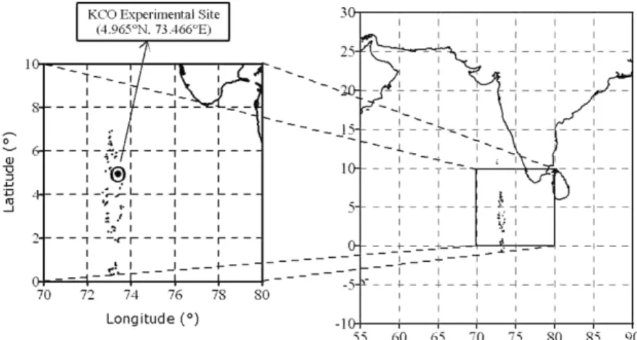
Kaashidhoo is an isolated, small and falcate shaped island, roughly 2.9 km by 1.0 km, in the Republic of Maldives, approximately 550 km southwest of the southern tip of the India. Maldives consists of a group of almost 1200 small islands forming a long, narrow belt spread over the Indian Ocean extending along the latitudinal region between

(3)

~7°N to ~1°S (Fig. 1). As part of the INDOEX campaign, the Center for Clouds, Chemistry and Climate (C4) established the KCO on the island of Kaashidhoo (4.96°N, 73.46°E; encircled in Figure 1) in the Republic of Maldives in the year 1998 (Moorthy and Satheesh 2001; Ramanathan et al. 2001; Satheesh et al. 1999). This Observatory provides the facilities to record standard meteorological observations such as wind speed and direction, dry air temperature, relative humidity, barometric pressure and rainfall. Database used in the study

During the INDOEX, IFP-99 campaign, two types of meteorological observations were carried out over Kaashidhoo: (1) surface layer meteorological observations taken from a 14-m meteorological tower mounted at KCO and (2) upper air meteorological observations obtained from balloonborne GPS Loran Atmospheric Sounding (GLASS) system. GLASS Sonde launches were conducted on regular basis at KCO from February 11 to March 29, 1999. On an average, daily three launches were made at 00:00, 06:00 and 12:00 UTC (corresponding to 05:00, 11:00 and 17:00 LT; KCO Local Time = GMT + 05:00 Hrs). On some specific days, soundings were also conducted at 18:00 UTC (corresponding to 23:00 LT). Overall, 143 soundings were conducted during the campaign. In the present study, surface layer observations and vertical profiles of meteorological parameters obtained from GLASS Sonde launches are used for setting the initial conditions of the ARPS model. Model simulations were carried out for 24 hours in vertical column mode configuration for obtaining the profiles of winds, potential temperature and specific humidity and to understand the impact of surrounding ocean on the diurnal evolution of the ABL over Kaashidhoo.

3. Numerical Simulations over Kaashidhoo during

INDOEX, IFP-99

The ARPS model has been developed by the Center for Advanced Prediction of Storms, Norman, Oklahoma, USA. ARPS is a three dimensional, non-hydrostatic and fully compressible, primitive equation model designed for storm and mesoscale atmospheric simulation and real time prediction (Xue et al. 1995). It uses a generalized terrainfollowing co-ordinate system with equal spacing in x- and y- directions and grid stretching in the vertical. Depending on the choice of Users and availability of lateral boundary conditions, ARPS

can be configured in one-, two- and three-dimensional modes. For two- and three-dimensional configuration, the model requires accurate lateral boundary conditions and fine topography details, which at present are not available for the KCO experimental site. The mesoscale model ‘ARPS’ has a salient feature that the base state of the model variables can be initialized through a single sounding profile and timedependent fields can be opted for self-initialization using analytic functions. Keeping the limitations of data availability and lateral boundary conditions over KCO, the ARPS model is configured in one-dimensional mode for simulation of vertical profiles of winds, temperature and humidity, so that the simulated output can be compared with the actual observations. All the simulations are done for duration of 24 hours, and the models are initialized with vertical profiles of meteorological parameters corresponding to 0600 UTC GLASS Sonde sounding. Table 1 shows the modelrun configuration of ARPS indicating some important parameters fed to the model:

4. Methodology of Data Assimilation through

Nudging

Data assimilation through nudging: a general introduction In numerical simulations through a model, prognostic variables are solved in time and space domain. Initially, a known set of values are assigned to the prognostic variables (initial conditions) and then with due passage of time, model variables are evaluated forward in time. For improving the quality of model simulations, one needs to incorporate different data assimilation techniques in the model, so as to provide the model realistic information through the observational data. In a broad sense, ‘Data Assimilation’ can be defined as the technique whereby

Table 1. ARPS Model Configuration

Model Configuration 1-D vertical column mode Model domain center Kaashidhoo (04.96°N, 73.46°E)

Time step 60 seconds

Terrain Option No terrain, flat ground

Mean sea level 5.0 m

Model grid set up vertical grid stretching

Soil type sandy loam

Roughness length for momentum 0.001 m Roughness length for heat 0.001 m

(4)

observational data are combined with output from a numerical model to produce an optimal estimate of the evolving state of the system. Thus, data assimilation at regular intervals will provide the model a guiding path, so as to keep the model forecasts always closer to the observations. In the present analysis, we make use of Nudging technique for incorporation of observational data in model simulations. Through this technique, we firstly identify the assimilation window in space and time over which the observational datasets need to be inserted and the model products require to be adjusted. Appropriate model variables are then adjusted for the realistic observational datasets with a proper weight being given to the observations.

Defining the assimilation window

In general, model variables are solved in time and space domain. Initially, the model is given some known set of values to these variables and then with due passage of time, model variables are evaluated forward in time. To make the concept more clear, let us assume that ‘Amod (x, y, z, t)’ is a

model variable, which is function of space (xmod = east-west

direction; ymod= north-south direction; zmod= vertical direction)

and time (tmod= time). The model can be initialized by

assigning some known values to variable ‘Amod’ at model

grid-points. As, the model simulations in the present analysis

are carried out in one-dimensional configuration, we simplify our assumptions by ignoring the xmod- and ymod- variations

in Amod. Thus, Amod can be redefined as a function of zmod

and tmod, i.e. ‘Amod (zmod, tmod)’. In the present configuration

of ARPS, the model has 33 vertical layers (i.e. zmod varies

from 1 to 33) and tmod varies in steps of 60 seconds (i.e.

model time step is = 60 seconds). Hence, in model simulation of 24 hours, ‘Amod (zmod, tmod)’ will have 1441

snapshots: every snapshot with 33 different values of variable ‘Amod’in vertical (Fig. 2).

Let us now assume that we have observational dataset ‘Aobs (zobs, tobs)’ corresponding to the model variable ‘Amod

(zmod, tmod)’ for a given timestamp, say: tobs = 12 hrs. It has to

be noted that observational grid points in zobs and tobs can be

different from the model grid points, i.e. zmod and tmod. Our

aim is to incorporate the observational data in model simulations through nudging technique; therefore, we first interpolate the observational dataset Aobs (zobs, tobs) to the

model grid points, i.e., mapping of Aobs (zobs, tobs) to Aobs (zmod,

tmod). This task is achieved by simple linear interpolation of

the variables. Once the observational data Aobs is interpolated

to model grid points, we define a temporal window, extending to a width of Δt in time on either side of t_obs. Such a window extending to t on either side of the observational timestamp tobs is referred to as assimilation window in time

(See Fig. 3):

Fig. 2. Pictorial representation of evolution of model variable A (z, t) in time. Here time varies from 60 seconds to 24 hrs in time-step of 60 seconds. Model configuration has 33 layers in vertical.

Fig. 3. Pictorial representation of data assimilation window in time. Observational data point is available at t = 12 Hrs. Y-axis shows the percentage of alteration in model variables for the corresponding time.

(5)

(tobs - Δt) ≤ t ≤ (tobs + Δt) (1)

Choice of the data assimilation time-window is indeed a trivial task. In the present case of data assimilation, we have made use of vertical soundings through GLASS Sonde which has got a typical ascent rate of about 4 to 5 m/s. Thus, a vertical sounding up to an altitude of 5 kms will take approximately 16 to 21 minutes. In order to avoid any sudden and rapid perturbations in atmospheric parameters, we have taken these profiles (obtained within a duration of about 20 minutes) to represent a time-window of about 60 minutes, which seems to be scientifically significant and acceptable.

Alteration in model variables through nudging: equations Now, we define the equations involved in the data assimilation scheme for alteration of model variables in the assimilation window. For a given time-stamp, t = t1, the ‘innovation’ in the model variable Amod (difference between

the model variable and observations) two can be written as: dA (z, t1) = Amod (z, t1) – Aobs (z, t1) (2)

In a crude way, the above equation representing the model innovation is one of the indirect measures of model errors, because the actual error is defined as the difference between the model variable and the truth. It has to be noted that the observations cannot be taken to be the truth, as it may have its own observational error (including instrumental and spatial representation error). If the model innovation term ‘dA’ is positive, it indicates that model is overestimating this variable, whereas negative values of dA indicate underestimation by the model. In either case, we need to adjust the model variables, so as to minimize the error dA. However, model variables cannot be altered drastically for a given location, as it can introduce some other errors in related variables and the chances of model blowing out increases. Therefore, a slight modification in model variables is recommended. In the data assimilation scheme suggested here, we alter the model variables through the following equation:

Anew (z, t1) = Amod (z, t1) + Δw (t1).dA (z, t1) (3)

In the above equation (3), Anew (z, t1) indicates the modified

(altered) model variables, whereas Δw (t1) is weighting function, which is taken to be function of time. The weighting function Δw (t) is taken to be maximum at

observational timestamp, and it is set to decay for timestamps away from the observational timestamp in Gaussian manner. The choice of weighing function generally depends on the possible tolerance limit of the parameters' variability. For example, if we need to determine a weighing function for the alterations in relative humidity, we may have to always restrict the variability within a permissible range of 0% to 100%; thus we have constraints on choice of weighing function. In case of other parameters, we have carried out a trial-and-error exercise by restricting the variability within one to two times of standard deviation of the concerned parameter in vertical. As such, there is no rockrigid rule that we should not alter the prognostic variables beyond some limit, but if similar exercise is done in 3-D configuration, it will create instability in model simulations, thereby introducing the possible constraints in the choice of weighing function. In the present case, through trial and error method, we have fixed the weighting function as 0.5 at observational timestamp. In the present analysis, data assimilation window is taken to be one hour. Equation (3) is extended over the entire data assimilation window, as defined in equation (1). Testing of nudging algorithm on ARPS for Kaashidhoo data

Availability of high resolution profiles of ABL parameters at a regular interval over Kaashidhoo Island during INDOEX, IFP-99 campaign enabled us to test the data assimilation scheme through nudging and to compare the model simulations with the observations. Due to unavailability of lateral boundary conditions and other flux related fields, ARPS model was customized for 1-D configuration over Kaashidhoo (Subrahamanyam, 2003; Subrahamanyam et al., 2006). Model simulations were carried out for duration of 24 hours each for an individual run starting from 06:00 UTC to 06:00 UTC (next day). Vertical profiles of meteo-rological parameters corresponding to 06.00 UTC soundings were used for initializing the model, while the profiles corresponding to 12.00 UTC soundings were injected in the model simulations through the nudging technique mentioned in this section. Model simulated profiles of ABL parameters corresponding to 12:00 (+6 Hrs), 18:00 (+12 Hrs) and 24:00 UTC (+ 18 Hrs) were compared with the available soundings data.

In real practice, there is good scope for alteration of the above equations. While we consider the two-dimensional space in horizontal, we can also define another weighting

(6)

function in space in a similar fashion, as that in equation (3). Through this scheme, model variables are adjusted towards the observations and bring the model simulations closer to the observations. To incorporate the above scheme in ARPS, we have injected a data assimilation subroutine in the main code of the model between two consecutive time step calculations of the model variables. Firstly, the model time is checked for whether it falls within the assimilation window or not. If the model time does not fall in assimilation window, then model variables are not altered. But for the model variables falling within the data assimilation window, appropriate changes are done as mentioned above.

5. Results and Discussion

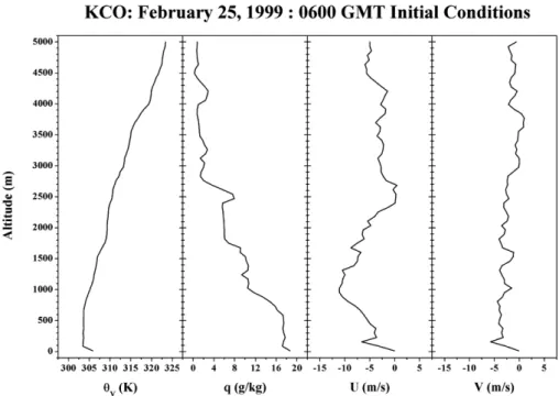
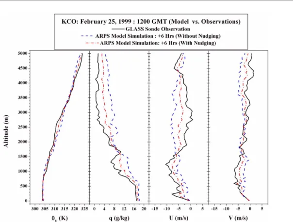
In Figure 4, we show typical profiles of virtual potential temperature (θ_V), specific humidity (q), zonal and meridional (U- and V-) wind components obtained from GLASS Sonde launch on February 25, 1999 (06:00 UTC). This data was used for generation of initial conditions to the ARPS model and simulations were carried out for next 24 Hrs. In Figures 5, 6 and 7, we show comparison of model simulated profiles with the GLASS Sonde observations corresponding to 12:00, 18:00 and 24:00 UTC respectively. Based on the profiles shown in Figures 5, 6 and 7, the Root Mean Square (RMS) errors for virtual potential temperature (θ_V), specific

humidity (q), zonal and meridional (U- and V-) wind components are tabulated in the following Table 2. From the Figures 5, 6 and 7 and Table 2, we notice that - Nudging of observational data in ARPS improve the RMS errors in model parameters significantly for the simulations corres-ponding to 12:00 and 18:00 UTC (i.e. +6 and +12 Hrs: Figures 5 and 6) respectively, however its impact is almost negligible for model simulations corresponding to 00:00 UTC (i.e. +18 Hrs: Figure 7). As the model time progresses ahead of the time of observations (in present case, 12:00 UTC), impact of nudging gradually vanishes. In the present case, model products for +18 Hrs simulations after incorporation of nudging are similar to the one obtained without incorporating nudging equations (Figure 7).

In the present work, since the ARPS model was run in one-dimensional configuration, its simulations will have their own limitations. One-dimensional configuration runs of model will not be able to capture horizontal advection of an air-mass and therefore may not be particularly useful for long-range forecasts; however, keeping in mind the data scarcity over such a tiny island, the results are significant in themselves that in one-dimensional configuration, nudging of vertical profiles of meteorological parameters did improve simulations to a reasonable extent, providing the scope of the data assimilation algorithm over various regions, where data limitation is one of the constraints in model simulations.

Fig. 4. Profiles of virtual potential temperature (θV), specific humidity (q), zonal and meridional (U- and V-) wind components corresponding to February 25, 1999-06:00 UTC.

(7)

Fig. 5. Comparison of model simulated (+6 Hrs) virtual potential temperature (θV), specific humidity (q), zonal and meridional (U- and V-) wind component profiles for 12:00 UTC with the GLASS Sonde observations.

(8)

The method described in this article is a probable way to improve initial conditions of the model and therefore holds promise for future research.

6. Concluding Remarks

In this article, we presented a new data assimilation scheme based on optimal interpolation and nudging concepts. The new scheme is based on the fact that model simulations can be brought closer to the observations by biasing the model simulations towards the observations with intermittent alteration in the model variables. Such a technique can serve to be a very good tool, where ample number of observational datasets is available. In this piece of research,

due to lack of observational datasets in large spatial domain, the nudging technique has been tested only for one-dimensional configuration and the study can be extended to spatial domain, where we have good knowledge of all model parameters in three-dimensional configuration. Through trial and error, we notice that intermittent data assimilation certainly improved the quality of model simulations for ABL parameters to a time domain of about +12 Hrs; however, the impact of nudging was not eminent for simulations corresponding to +18 Hrs. Keeping the constraints of one-dimensional model configuration used in the present study, there is ample scope for improvements in the nudging equations shown in the present article; nonetheless the nudging technique proves to be a very

Table 2. RMS Errors in model simulations Sl. No. Parameter +06 Hrs +12 Hrs +18 Hrs Without Nudging With Nudging Without Nudging With Nudging Without Nudging With Nudging 1. Virtual potential temperature (θV, in deg. K) 1.1429 0.5715 0.5767 0.4037 0.6791 0.6282 2. Specific humidity (q, in g/kg) 1.9869 .9934 3.0515 2.1360 2.1197 1.9607 3. Zonal wind component (U-, in m/s) 4.2871 2.1436 1.3896 0.9728 2.0403 1.8873 4. Meridional component (V-, in m/s) 2.7367 1.3683 1.8033 1.2623 1.8469 1.7084

(9)

useful tool for improving the model simulations within a mesoscale domain.

Acknowledgements

We are very much thankful to Dr. Tuhin Kumar Mandal, National Physical Laboratory, New Delhi for providing the GLASS Sonde data over Kaashidhoo for this piece of research. We are also thankful to all the persons who were directly or indirectly involved in carrying out the KCO component of INDOEX, IFP-99 campaign successfully. We would also like to extend our sincere thanks to Prof. R. Sridharan for his consistent encouragement for carrying out atmospheric modelling activities at SPL, VSSC. One of the authors, S. Indira Rani is thankful to Indian Space Research Organization for providing research fellowship for carrying out her Ph.D work.

References

Anthes, R.A. 1983. A review of regional models of the atmosphere in middle latitudes. Mon. Weather Rev., 111, 1306-1335. Moorthy, K.K. and S.K. Satheesh. 2001. Aerosol characteristics

over minicoy: Evicence of influence of mineral dust transport. J. Mar. Atmos. Res., 2, 26-32.

Pielke, R.A. 1984. Mesoscale Meteorological Modeling. Academic Press Inc., Orlando, Florida.

Ramanathan, V., P. Crutzen, J. Lelieveld, A. Mitra, D. Althausen,

J. Anderson, M. Andreae, W. Cantrell, G. Cass, C. Chung, A. Clarke, J. Coakley, W. Collins, W. Conant, F. Dulac, J. Heintzenberg, A. Heymsfield, B. Holben, S. Howell, J. Hudson, A. Jayaraman, J. Kiehl, T. Krishnamurti, D. Lubin, G. McFarquhar, T. Novakov, J. Ogren, I. Podgorny, K. Prather, K. Priestley, J. Prospero, P. Quinn, K. Rajeev, P. Rasch, S. Rupert, R. Sadourny, S. Satheesh, G. Shaw, P. Sheridan, and F. Valero. 2001. The Indian Ocean experiment: An integrated analysis of the climate forcing and effects of the great Indo-Asian haze. J. Geophys. Res., 106(D22), 28371-28398.

Satheesh, S.K., V. Ramanathan, X. Li-Jones, J.M. Lobert, I.A. Podgorny, J.M. Prospero, B.N. Holben, and N.G. Loeb. 1999. A model for the natural and anthropogenic aerosols over the tropical Indian Ocean derived from Indian Ocean Experiment data. J. Geophys. Res., 104(D22), 27421-27440. Subrahamanyam, D.B. 2003. Observational and modelling studies of the marine atmospheric boundary layer over the tropical Indian Ocean during INDOEX. Ph.D. Thesis, Mahatma Gandhi University, India. 175 p.

Subrahamanyam, D.B., R. Radhika, and P.K. Kunhikrishnan. 2006. Improvements in simulations of atmospheric boundary layer parameters through data assimilation in ARPS mesoscale atmospheric model. p. 64040K1. In: Proc. SPIE, Remote sensing and modeling of atmosphere, oceans and interactions. Vol. 6404.

Xue, M., K.K. Droegemeier, V. Wong, A. Shapiro, and K. Brewster. 1995. ARPS version 4.0 User’'s guide. CAPS, NSF, FAA, University of Oklahama, USA. 380 p.