1. INTRODUCTION
Major characteristic of the industrial systems is that there are various constraints including the long dead time and constant system, the multi-variable system, nonlinear system, and non-minimum phase system.
The effective measurement of industrial system is needed for system identification about long-range dead-time system among system constraints.
The performance and the stability of time-delay process are influenced by dead time. To solve the constraints, the smith predictor, that has the compensation of dead time and the matched model, was proposed.[1]
In good model case, the merits of the smith predictor include the ability to improve the performance and to disregard the dead time caused by the characteristics of closed-loop system. But, to apply the smith predictor effectively, the model must be matched with the real system. If the model is mismatched with the system, the smith predictor is difficult to be applied in the real industry.
Thus, the system identification is very important in time-delay process. The systems for identification could be divided into linear and nonlinear types. But, this study divided into it two types: FOPDT(First Order Plus Dead Time) system and SOPDT(Second Order Plus Dead Time) system which are mainly used in the industry.
For system identification methods about real industrial system, the input signal can have significant on identification results. Generally, test signals include pseudo-random binary sequence, pulse, step, ramp, and sinusoidal functions. But, the step test of all these tests is the simplest, needs little equipment, and can even be performed manually.
In this paper, we reviewed the identification methods that are area-based identification and direct identification for time-delay process. And we proposed the real-coded genetic
algorithm for identification of FOPDT and SOPDT processes.
2. IDENTIFICATION METHODS 2.1 Area-based Identification
The first-order plus dead-time(FOPDT) model which describes a linear monotonic process quite well in most chemical process is applied as an approximation to such processes.
This model is able to represent as equation (1)[2].
)
(
1
)
(
e
U
s
Ts
K
s
Y
−Ls+
=
(1)where K, T, L are the process gain, the time constant, and the dead time respectively.
A graphical method is the simplest method of all the identification methods. The intercept of the tangent to the step response that has the largest slope with respect to the horizontal axis gives L. T is determined from the difference between L and the time when the step response reaches the value of 0.63K. And, the times at which the process output reaches 28% of K and 63% of K, respectively, are measured, and used to estimate T and L. These two methods are simple, but quite sensitive to large measurement noise. Thus, an area-based method has been proposed as better estimation robustness[3].
The process gain K is obtained from the steady states of the process input and output. The average residence time is computed from the area in Figure 1.
Real-coded genetic algorithm for identification of time-delay process
Gang-Wook Shin*, and Tae-Bong Lee*** Korea Institute of Water and Environment, KOWACO, Daejeon, Korea (Tel : +82-42-860-0413; E-mail: [email protected])
**Dept. of Electronics Information Eng, Kyungwon College, Gyeonggi do, Korea (Tel : +82-31-750-8755; E-mail: [email protected])
Abstract: FOPDT(First-Order Plus Dead-Time) and SOPDT(Second-Order Plus Dead-Time) process, which are used as the most useful process in industry, are difficult about process identification because of the long dead-time problem and the model mismatch problem. Thus, the accuracy of process identification is the most important problem in FOPDT and SOPDT process control. In this paper, we proposed the real-coded genetic algorithm for identification of FOPDT and SOPDT processes. The proposed method using real-coding genetic algorithm shows better performance characteristic comparing with the existing an area-based identification method and a directed identification method that use step-test responses. The proposed strategy obtained useful result through a number of simulation examples.
Keywords: Genetic algorithm, Identification, time-delay, FOPDT, SOPDT
K A0
Tar
A1
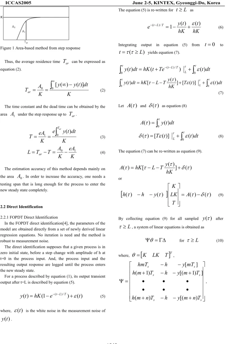
Figure 1 Area-based method from step response
Thus, the average residence time
T
ar can be expressed as equation (2).K
dt
t
y
y
K
A
T
ar∫
∞−
∞
=
=
0 0[
(
)
(
)]
(2)The time constant and the dead time can be obtained by the area
A
1 under the step response up toT
ar.K
dt
t
y
e
K
eA
T
ar T∫
=
=
1 0(
)
(3)K
eA
K
A
T
T
L
=
ar−
=
0−
1 (4)The estimation accuracy of this method depends mainly on the area
A
0. In order to increase the accuracy, one needs a testing span that is long enough for the process to enter the new steady state completely.2.2 Direct Identification 2.2.1 FOPDT Direct Identification
In the FOPDT direct identification[4], the parameters of the model are obtained directly from a set of newly derived linear regression equations. No iteration is need and the method is robust to measurement noise.
The direct identification supposes that a given process is in zero initial state, before a step change with amplitude of h at t=0 in the process input. And, the process input and the resulting output response are logged until the process enters the new steady state.
For a process described by equation (1), its output transient output after t=L is described by equation (5).
)
(
)
1
(
)
(
t
hK
e
( )/t
y
=
−
−t−L T+
ε
(5) where,ε
(t
)
is the white noise in the measurement noise of)
(t
y
.The equation (5) is re-written for
t ≥
L
ashK
t
hK
t
y
e
−(t−L)/T=
1
−
(
)
+
ε
(
)
(6)Integrating output in equation (5) from
t
=
0
to)
(
L
t
=
τ
τ
≥
yields equation (7).∫
τ=
+
− − τ+
∫
τε
0 0 / ) ()
(
)
(
)
(
t
dt
hK
t
Te
t
dt
y
L T L t∫
τ=
τ
−
−
τ
+
ε
τ+
∫
τε
0]
[
(
)]
0(
)
)
(
[
)
(
T
t
t
dt
hK
y
T
L
hK
dt
t
y
L (7)Let
A
(
τ
)
andδ
(
τ
)
as equation (8)∫
=
ττ
0(
)
)
(
y
t
dt
A
∫
+
=
ε
τ τε
τ
δ
0(
)
)]
(
[
)
(
T
t
t
dt
L (8)The equation (7) can be re-written as equation (9).
)
(
]
)
(
[
)
(
τ
=
τ
−
−
τ
+
δ
τ
hK
y
T
L
hK
A
or[
(
τ
)
(
τ
)
]
=
(
τ
)
−
δ
(
τ
)
−
−
A
T
LK
K
y
h
h
(9)By collecting equation (9) for all sampled
y
(
τ
)
afterL
≥
τ
, a system of linear equations is obtained asΓ∆
=
Ψ
θ
forτ
≥
L
(10) where,θ
=
[
K
LK
T
]
T,
+
−
−
+
•
•
•
•
•
•
+
−
−
+
−
−
=
Ψ
s s s s s sT
n
m
y
h
T
n
m
h
T
m
y
h
T
m
h
mT
y
h
hmT
)
[(
)
(
]
)
1
[(
)
1
(
]
[
,
+
•
•
+
=
Γ
]
)
[(
]
)
1
[(
]
[
s s sT
n
m
A
T
m
A
mT
A
,
+
−
•
•
+
−
−
=
∆
]
)
[(
]
)
1
[(
]
[
s s sT
n
m
T
m
mT
δ
δ
δ
sT
is the sampling interval andmT
s≥
L
. The estimationθ
ˆ
ofθ
in (10) can be obtained using the least-squaresmethod as
Γ
Ψ
Ψ
Ψ
=
(
T)
−1 Tˆ
θ
(11) 2.2.2 SOPDT Direct IdentificationA stable SOPDT process can be represented in the Laplace domain by equation (12) and in time domain by equation (13) under zero initial conditions with the time delay,
L
≥
0
.)
(
)
(
)
(
)
(
2 1 2 2 1e
U
s
a
s
a
s
b
s
b
s
U
s
G
s
Y
−Ls+
+
+
=
=
(12))
(
)
(
)
(
)
(
)
(
t
a
1y
t
a
2y
t
b
1u
t
L
b
2u
t
L
y
&
+
&
+
=
&
−
+
−
&
(13)
Integrating both sides of equation (13) is expressed equation (14).
∫
+
∫ ∫
+
a
ty
d
a
ty
d
d
y
0 2 0 0 1 1 1(
)
(
)
ττ
τ
τ
τ
τ
∫
−
+
∫ ∫
−
=
b
tu
L
d
b
tu
L
d
d
0 2 0 0 1 1 1(
)
(
)
ττ
τ
τ
τ
τ
(14) (4.16) Assume that the input is of step type with magnitude h,)
(
1
)
(
t
h
t
u
=
•
, where0
)
(
1
t
=
ift
〈
0
1
)
(
1
t
=
ift
≥
0
∫
tu
−
L
d
=
t
−
L
h
0(
τ
)
τ
(
)
∫ ∫
tu
−
L
d
d
=
t
−
L
h
0 0 2 1 1(
)
2
1
)
(
ττ
τ
τ
(15)Equation (16) is yielded by substituting (15) into (14).
∫
−∫ ∫
+ − + − − = a ty d a t y d d b t Lh b t L h y 0 0 0 2 2 1 1 1 2 1 ( ) 2 1 ) ( ) ( ) (τ τ τ τ τ τ∫
−∫ ∫
+ − + + − + − = t t h t b th L b b h L b L b d d y a d y a 0 0 0 2 2 2 1 2 2 1 1 1 2 1 2 1 ) ( ) 2 1 ( ) ( ) (τ τ τ τ τ τ (16))
(t
γ
,φ
T(t
)
,θ
T can be respectively defined as equation (17).)
(
)
(
t =
y
t
γ
− − =∫
y d∫ ∫
y d d h th t h t t t T 2 0 0 1 1 0 2 1 ) ( ) ( ) (τ
τ
ττ
τ
τ
φ
−
+
−
=
1 2 2 2 2 1 2 12
1
b
L
b
b
L
b
L
b
a
a
Tθ
(17)Then equation (16) can be expressed as (18) by using equation (17).
θ
φ
γ
(
t
)
=
T(
t
)
(18) Chooset
i , such thatL
≤
t
1〈
t
2〈
L
〈
t
N , and let[
γ
(
t
1)
γ
(
t
2)
L
γ
(
t
N)
]
=
Γ
and[
]
T Nt
t
t
)
(
)
(
)
(
1φ
2φ
φ
L
=
Φ
. Then equation (18) is expressed as equation (19).θ
Φ
=
Γ
(19)One can readily see that the columns in
Φ
are independent, andΦ
TΦ
is nonsingular. Thus, the ordinary least squares(LS) can be applied to equation (19) to findθ
ˆ
, an estimate ofθ
by (20).Γ
Φ
Φ
Φ
=
(
T)
−1 Tˆ
θ
(20) 3. Real-Coded Genetic Algorithm3.1 Simple Genetic Algorithm
Simple Genetic Algorithm(SGA) generally consists of individual initialization, fitness evaluation, and new population showed in figure 2.
The way to represent points on search space in SGA uses the binary encoding or the binary coding as most general methods.
According to this way, initialization methods, which make initial individual population for simulated evolution, include the random initialization and the directed initialization based on prior knowledge or experience.
Individual Initialization Fitness Evaluation END Yes Termination Condition Selection Operator Crossover Operator Mutation Operator No New Population
Figure 2. Flow chart of simple genetic algorithm
Adaptability of GA changes based on fitness evaluation of individuals like adaptability of lives does under the circumstance of the natural world. Whenever a new population forms, fitness of each individual is evaluated using objective function.
To create a new population is to make a new offspring of next generation by selection, crossover, and mutation operation based on strings of chromosomes.
Selection operator is a procedure that reproduces the individual by fitness of each individual. In natural world, offsprings have genes transmitted from parents but in some way their characters differ with those of parents. Imitation of above procedure in genetic algorithm is crossing procedure.
Mutation provides new information that is not existted in present population. The optimization of SGA finishes whenever new individuals through these procedures satisfies proper convergence condition or whenever proper iterations finish
3.2 Proposed Genetic Algorithm
GA chromosomes could be generally represented as equation (21). Forms of each gene are binary in simple genetic algorithm and real-number in real-coded genetic algorithm.
Also, demerits of binary gene could be complemented by changing binary to real-number.
{
i i i in}
i
x
x
x
x
S
=
1 2 3L
(21)where
S
i is i-th chromosome of population,x
in is n-th gene of i-th chromosome.In some vector
x ∈
R
n, the lengthl
of chromosomei
S
is as same as vector dimensionn
.Real-coded algorithm is a typical expression that can solve above problems by easily designing the tools to treat constraints and the operators with knowledge related to the problems, using a way that make the chromosome expression approach more closely to the solution space.
Although arithmetic crossover that relaxes discontinuity at crossover point is used the most frequently in real-coded crossover methods, the search space of the crossover can be reduced by limited range of multiplier that is a main factor of the first combination between parent chromosomes.
So, follow equation (22) proposes the modified crossover operator to extend the multiplier range along with fitness of parent chromosomes. 2 1 1
(
1
)
ˆ
x
x
x
=
λ
s+
−
λ
s (22a) 1 2 2(
1
)
ˆ
x
x
x
=
λ
s+
−
λ
s (22b) If chromosomes of two parents areS
1 andS
2 and the relationship between their fitnessesf
(
S
1)
andf
(
S
2)
isf
(
S
1)
≥
f
(
S
2)
, the range ofλ
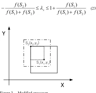
s could be set as equation (23). The initial search ability to seek for global solution is increased by extending the search range of the chromosome which has larger fitness.)
(
)
(
)
(
1
)
(
)
(
)
(
2 1 1 2 1 2S
f
S
f
S
f
S
f
S
f
S
f
s+
+
≤
≤
+
−
λ
(23) S2(x2,y2) S1(x1,y1)X
X
X
X
Y
Y
Y
Y
Figure 3. Modified crossover
Cost function is calculated to minimize the variance between the step input response and the reference. Fitness
)
(
S
if
evaluation is calculated by cost functionJ
(
S
i)
of each chromosomeS
i, and can be calculated by transforminginto maximization problem as equation (24).
α
+
=
)
(
1
)
(
i iS
J
S
f
(24)where
α
is a constant that the fitness values are always positive,α
is set at 0.1 not to make it divided by 0 in this study.4. SIMULATIONS 4.1 FOPDT Process
The identification parameters of FOPDT process are defined as three parameters, which are genes of GA chromosomes: process gain, time constant, and dead time.
Individual initialization is a method that each chromosome randomly takes a point in domain to be a point in proper area. In FOPDT process identification, however, individual initialization randomly takes a point in domain using output response by initial step input as follows.
final final
ocess
Gain
Y
Y
≤
≤
×
×
Pr
_
1
.
2
8
.
0
2
/
_
tan
_
0
≤
Time
Cons
t
≤
Rise
Time
(25) ) 1 . 0 ( _0≤Dead Time≤ ×Yfinal
To identify FOPDT process, detail design parameters of proposed real-coded GA are represented in Table 1.
Table 1. Parameters of real-coded GA
Population number 40
String length 3
Generation number 100
Crossover probability 0.9 Mutation probability 0.05
Crossover method Modified convex Selection method Tournament Mutation method Modified real-number creep
To verify the validity of process identification using GA, each process of four types compares relationship among results made by three different identification methods : area-based identification, directed identification and proposed GA identification.
The systems considered for simulation are FOPDT process equation (26), SOPDT process equation (27), non-minimum
phase process equation (28), and multi-lag process equation (29). The equations of the processes are represented as follows.
1
)
(
+
=
−s
e
s
G
s (26))
1
2
)(
1
10
(
)
(
4+
+
=
−s
s
e
s
G
s (27) 5)
1
(
1
)
(
+
−
=
s
s
s
G
(28) 8)
1
(
1
)
(
+
=
s
s
G
(29)To obtain the time-domain identification error for step input of each process, equation (30) is used to calculate the square means of error between the actual process output and the estimated output.
∑
+ =−
+
=
m n m k s sy
kT
kT
y
n
2)]
(
ˆ
)
(
[
1
1
ε
(30)where
y
(
kT
s)
is the actual process output under a step change, andy
ˆ
(
kT
s)
is the response of the estimated process under the same step change.
Table 2 Comparison of results from identification methods for FOPDT
Processes
G
(s
)
Identified processesG
ˆ s
(
)
Errorε
Area method 1 99 . 0 01 . 1 + − s e s 70828
.
2
e
− Direct method 1 997 . 0 + − s e s 82534
.
2
e
− 1 + − s es Proposed 1 999 . 0 + − s e s 95012
.
2
e
− Area method 1 19 . 10 83 . 5 + − s e s 52598
.
4
e
− Direct method 1 41 . 11 03 . 1 5.47 + − s e s 45042
.
4
e
− ) 1 2 )( 1 10 ( 4 + + − s s e s Proposed 1 52 . 10 67 . 5 + − s e s 54717
.
3
e
− Area method 1 11 . 2 4 + − s e s 41767
.
2
e
− 5 ) 1 ( 1 + − s s Direct method 1 45 . 2 01 . 1 3.73 + − s e s 49714
.
1
e
−Proposed method 1 5 . 2 6 . 3 + − s e s 4
2435
.
1
e
− Area method 1 3 . 4 3 . 4 + − s e s 41414
.
5
e
− Direct method 1 81 . 3 06 . 1 4.94 + − s e s 30000
.
3
e
− 8 ) 1 ( 1 + s Proposed 1 5 . 3 99 . 0 4.7 + − s e s 42383
.
4
e
−Judging from simulation results about error value of each process, response characteristics by area-based identification and those by directed identification were similar, but the results obtained by proposed identification were better than those by other methods.
Among four types of processes, identification error was similar in all three methods only for FOPDT process. Identification error of area-based and directed identification methods was greater than that of proposed method for three other processes: SOPDT process, non-minimum phase process and multi-lag process.
4.2 SOPDT 4.2 SOPDT 4.2 SOPDT 4.2 SOPDT ProcessProcessProcessProcess
The input parameters for identification of SOPDT process consist of four parameters as equation (31). Four input parameters as equation (32) are represented as down-to-four-points of real-number. Ls
e
s
T
s
T
K
−+
+
21
2 1 (31)}
,
,
,
{
i 1i 2i i iK
T
T
L
S =
(32)To identify SOPDT process, detail design parameters of proposed real-coded GA were represented in Table 1.
Thus, to verify the validity of identification for SOPDT process like FOPDT process, the systems considered for simulation are equation (33) and equation (34).
5
)
1
(
1
+
s
(33) se
s
s
10 3 2)
1
2
(
)
1
(
08
.
1
−+
+
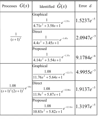
(34)Table 3, which is an error comparison table according to identification methods for two processes, verified that the validity of process identification of proposed GA was better than those of directed identification and graphic identification
Table 3 Result comparison from identification methods for SOPDT
Processes
G
(s
)
IdentifiedG
ˆ s
(
)
Errorε
Graphical s e s s 35 . 1 2 1 58 . 3 71 . 4 1 − + + 55237
.
1
e
− Direct s e s s 45 . 1 2 1 45 . 3 4 . 4 1 − + + 50947
.
2
e
− 5 ) 1 ( 1 + s Proposed s e s s 35 . 1 2 1 54 . 3 14 . 4 1 − + +9
.
1784
e
−6 Graphical s e s s 17 . 12 2 1 64 . 5 76 . 11 08 . 1 − + + 59955
.
4
e
− Direct s e s s 06 . 12 2 1 87 . 5 9 . 11 08 . 1 − + + 59137
.
1
e
− s e s s 10 3 2 ) 1 2 ( ) 1 ( 08 . 1 − + + Proposed s e s s 16 . 12 2 1 82 . 5 83 . 10 08 . 1 − + + 53197
.
1
e
− . 5. CONCLUSIONSReal-coded genetic algorithm was proposed on the identification of system parameters. To effectively apply the genetic algorithm to the identification, a modified crossover operator was proposed on selection of optimal parameters of system. By varying the multiplier to extend search space of existing crossover operator, the proposed operator makes a gene with larger fitness have greater chance of crossover. When the proposed operator was compared with the conventional crossover operator, excellent crossover characteristics were found from the proposed operator. This study compared the output responses obtained when step inputs were put into each process. The proposed identification obtained the best result in error rate of step response in comparison among area-based identification, directed identification, and proposed identification.
REFERENCES
[1]
O.J.M. Smith, “Closer control of loops with dead
time,” chem. Eng. Progress, Vol. 53, No. 5, pp.
217-219, 1957.
[2] K.J.Astrom and T.Hagglund, “PID controllers:theory, design, and tuning,” Instrument Society of Americae, 1995.
[3] A. Ingimundarson and T.Hagglund, “Robust tuning procedures of dead-time compensating controllers,” Control Engineering Practice, Vol. 9, pp. 1195-1208, 2001.
[4] Q.G.Wang and Y.Zhang, “Robust identification of continuous systems with dead-time from step responses,” Automatica, Vol.37, pp.377-390, 2001.