Reduction of GPS Latency Using RTK GPS/GNSS Correction and Map Matching in a Car NavigationSystem

1. Introduction

PND (Portable Navigation Device)‐type CNS (Car Navigation System), which have been distributed rapidly and used widely in the market, collect coordinate data from a GPS(Global Positioning System) receiver and display the current position of a car on a mapon the device’s screen (Ga et al.

2011). However, the difference between the definition time of the GPS position data and actual display time of the car position on the map could reduce the accuracy of the car position displayed. Because of the delayed processing, the car position that users see is no longer current by the time the GPS position has been determined. This is called the late processing problem and includes issues such as positional accuracy error and untimely navigation routing service. Because the positional difference due to the late processing problem could be tens of meters and

could include deviation from the driving course, an improved method to fix these problems is required for driving safety. It is expected that a method that uses predicted future positionsto compensate for the delay time caused by processing and displaying of received GPS signals, could mitigate these problems.

The inaccuracy of car positions on the CNS screen caused by delay in GPS signal processing and associated problems, has been a common issue dealt with by general navigation users and developers.

There have been numerous related studies to improve inaccuracy caused by late processing problems using Kalman filters. This is an effective technique for prediction of time series data including noise such as GPS receiver data.

In cases with no cars, Singer (1970) modeled a Kalman filter to use for the tracking of a manned maneuverable vehicle in a weapon system, and Friedland(1973) estimated positions and velocities of

Received: 2016.05.17, revised: 2016.06.22, accepted: 2016.06.24

* Deputy Manager, Energy & Chemical Business Team II, SK Holdings C&C, [email protected]

** Corresponding AuthorㆍMemberㆍAssistantProfessor, School of Convergence & Fusion System Engineering, Kyungpook National University, [email protected]

*** MemberㆍProfessor, Dept. of Civil & Environmental Engineering, Seoul National University, [email protected]

Reduction of GPS Latency Using RTK GPS/GNSS Correction and Map Matching in a Car NavigationSystem

1)

Kim, Hyo Joong*ㆍLee, Won Hee**ㆍYu, Ki Yun***

Abstract

The difference between definition time of GPS (Global Positioning System) position data and actual display time of car positions on a map could reduce the accuracy of car positions displayed in PND (Portable Navigation Device)‐

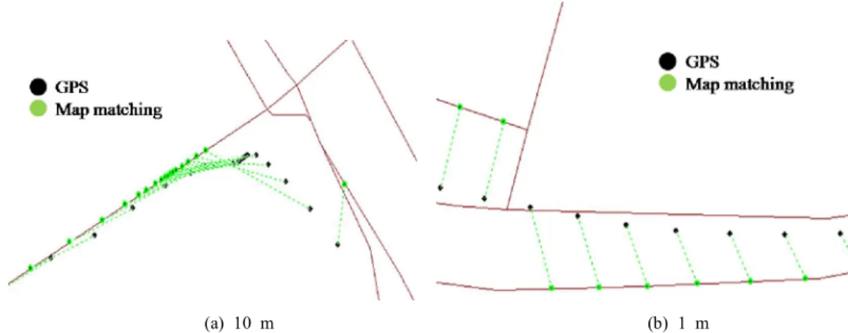
type CNS (Car Navigation System). Due to the time difference, the position of the car displayed on the map is not its current position, so an improved method to fix these problems is required. It is expected that a method that uses predicted future positionsto compensate for the delay caused by processing and display of the received GPS signals could mitigate these problems. Therefore, in this study an analysis was conducted tocorrect late processing problems of map positions by mapmatching using a Kalman filter with only GPS position data anda RRF (Road Reduction Filter) technique in a light‐weight CNS. The effects on routing services are examined by analyzing differences that are decomposed into along and across the road elements relative to the direction of advancing car. The results indicate that it is possible to improve the positional accuracy in the along‐the‐road direction of a light‐weight CNS device that uses only GPS position data, by applying a Kalman filter and RRF.

Keywords : Car Navigation System (CNS), Kalman Filter, Map Matching, Road Reduction Filter (RRF), Real‐

Time Kinematic (RTK), Global Positioning System (GPS)

37 Vol.24 No.2 June 2016 pp.37-46

Research Paper

ISSN: 2287-6693(Online) http://dx.doi.org/10.7319/kogsis.2016.24.2.037

moving objects when measuring position coordinates with a fixed time interval, including noise. In addition, related studies have been made in diverse fields such as prediction of human movements in computer vision (Kohler 1997), position tracking in wireless sensor and cellular networks (Yick et al.

2005; Takenga et al. 2007), and position tracking of storms (Manfredi et al. 2005). In the field of defining a robot system’s position, future positions of moving objects were predicted with a Kalman filter for time delay in the acquisition and processing of images during visual servicing (Gortcheva et al. 2001). As with cases including cars, Bonnifait et al. (2007) matched the resulting positions (corrected for GPS delay using a Kalman filter and with DR(Dead Reckoning) sensor data) to roads on a GIS (Geographic Information System)‐based map in the process of realizing a real‐time vehicle position estimation system. Tessier et al. (2006) predicted positions to compensate for GPS time delay in the process of integrating delayed observations from each sensor on a vehicle equipped with various sensors.

Tradisauskas et al.(2007) addressed the possibility of estimating the positions of a car on a roadmap several seconds ahead, considering the occurrence of delays caused by acquisition time of data from GPS/DR devices and processing time of map matching, but without describing the process or presenting experimental results.

From the studies mentioned above, most studies seem to be aimed at improving positional accuracy not only using GPS position data, but also by integratingit with data from other sensors for light weight hardware like PND. Map matching is a technique that determines approximate car positions on the roadmaps using GPS position data, including errors(Bernstein et al., 1996). RRF (road reduction filter), one of the commonly used map matching techniques, determines position by virtual differential GPS correction and eliminates improper candidate roads (Taylor et al. 2001). Similarly, there has been research regarding calculations of corrections from past matching results (Ahnet al. 2005; Xu et al.

2007). Quddus et al.(2003) analyzed the general map matching algorithms used in telematics

2. Method of prediction and processing of signals

2.1 Prediction using Kalman filter

A Kalmanfilter is an effective recursive filter that predicts the state of a dynamic system from measurements, including series of noise.A Kalman filter is essentially a set of mathematical equations that implement a predictor‐corrector type estimator that is optimal, in the sense that it minimizes the estimate error covariance. A Kalman filter model is described as an equation that represents the state at time step k by changes from the state at the previous time step as shown in Eq. (1).

1

1 -

-

+ +

=

k

Ax Bu w

x (1)

whereA is the state transition matrix that relates the previous state and the current state. B is the control input matrix applied to the control vector. Here, u .

w is the process noise and is assumed to have

normal distribution with average ‘0’ and covariance Q ⁽ p ⁽ w ^{) ~} N ^{( 0 ,} Q ⁾⁾ .

The measurement z

of the state x

at the time step K is represented as Eq. (2).

k k

k

Hx v

z _{= +} (2)

H is the measurement matrix that relates the state x and the measurement

z .

v is the measurement

noise. It is assumed to have normal distribution with

average ‘0’ and covariance ⁽ p ⁽ v ^{) ~} N ^{( 0 ,} Q ⁾⁾ . A

Kalman filter estimates a process using a form of

feedback control. That is, the filter estimates the

process state at some time and then obtains feedback

in the form of noisy measurements.It consists of two

stages, time update (predict) and measurement update

(correct).The time update equations are responsible

for projecting forward (in time) the current state and

error covariance estimates to obtain a priori estimates

for the next time step.The measurement update

equations are responsible for the feedback that is

used to incorporate a new measurement into the a

priori estimate to obtain an improved a posteriori estimate.To apply a Kalman filter to the estimation of the position coordinate of a moving car, a dynamic model of the car has to be established.According to Newton’s law, tracking the position and the velocity of a moving target, can be done with a two‐state dynamic model as in Eq. (3) (Friedland, 1973).

k k

k

Ax Ga

x =

+ (3)

When the measurement is taken at time period t D , it is assumed that the target is moving constantly with an arbitrary acceleration a

in the time between

- 1

k and k . The state transition matrix A and the matrix G that relates random noise is as Eq. (4).

ú ú ú ú

û ù

ê ê ê ê

ë é

D D

D D

= ú ú ú ú

û ù

ê ê ê ê

ë é

D D

=

t t

t t

t t

A / 2

2 / G 1 0 0 0

1 0 0

0 0 1 0

0 0 1

2

(4)

The acceleration added is assumed to be white noise and the covariance of it is given by Eq. (5).

ú ú ú ú ú

û ù

ê ê ê ê ê

ë é

D D

D D

D D

D D

=

=

2 2 3 2

3 2 4 2 2 2 3 2

3 2 4 2 2

2 / 0

0

2 / 4 / 0

0

0 0

2 /

0 0

2 / 4 /

t t

t t

t t

t t

GG Q

a a

a a

a a

a a

T a

s s

s s

s s

s s

s

(5)

2.2 Map matching using RRF

RRF(Road Reduction Filter) is a commonly used technique for map matching. As one of the techniques used to calculate the current position of a vehicle on a road map, it tracks the vehicle on all possible roads (road centerlines) in a computed error region (systematic error of GPS position data), and then uses a method of rapidly detecting inappropriate roads from the set of all those able to be removed.

Initial raw point position is computed using pseudo range measurements direct from a GPS receiverand VDGPS (Virtual Differential GPS)corrections are computed from previous positions. Height aiding with

DTM(Digital Terrain Model) is used to reduce the number of satellites required for a position solution.

Because it uses previous matching information to correct the current matching result, it is effective for branch roads and adjacent roads.However, it has several weaknesses, such as propagation of GPS signal error to create serious error in determination of position, especially for along road error and problems from changes in the road or turns at an intersection (Taylor et al., 2006).

To realize effective map matching, this study included additional factors in applying RRF. In the experiments the navigation system is within a car that is moving around in a downtown area, which is considered in determination of input or decision elements.

The critical values of filtering that remove inappropriate roads from the candidate roads, are set up as 5m for distance error and 45 degrees for bearing error, determined by searching for optimal values from experiments.If the critical value for distance error is too high, the sections of great change in direction, such as intersections,would not be recognized (as in Fig. 1(a)), andif too small, the current correct mapping road could be removed because in the real world the actual length traveled by a car and the corresponding length for the road on the map would never be same (as in Fig.

1(b)).Therefore, 5m is selected as the critical distance value: the maximum possible distance during one second of GPS receiving interval, when the car is driving at a general maximum speed of 60km/h (17m/s) in a down‐town area and the bearing difference between the road and the car is 45 degrees, the critical value of bearing error.

If the critical value of bearing error is too high, the sections of great change in direction such as intersections,would not be recognized, andif too small, current correct mapping road could be removed because it would become too sensitive to very small amounts of direction change from driving at low velocity or changing lanes, as shown in Fig.

2.

Figure 2. Possible problem by setting up the critical value of bearing error too small (30 degrees)

2.3 Development of test application

To organize the CNS environment, a test application that performs basic functions of navigation software was developed. It was developed with Visual C++ 6.0 language and provides several functions, such as receiving of GPS signals, parsing of GPS data, conversion of coordinates, Kalman filter, map matching, and displaying process results and maps.

The GPS receiver provides various GPS data formats, but NMEA(National Marine Electronics Association) 0183 standard GPRMC(Recommended Minimum Specific GNSS Data) format was used for this test application. The GPRMS format provides information such as latitude/longitude position, speed, direction, and signal generation time. Among these, UTC time data, status data, latitude/longitude field and checksum were used. For GPS status data, A and

V values are usable, but situations that do not guarantee validity of data received could happen for several reasons. Places like a tunnel or an underground passage where objects are blocking the top would be examples. In the case of A as status, the data received is valid if the GPRMC information is only used for post process. In the case of B as status, the data received is ignored. Data is also ignored when errors, like missing of message,are generated using checksum information.

The coordinates of the position on the roadmap resulting from the map matching algorithm based on RRF, is displayed on screen. The road map data is organized to basically create links between road intersections and vertexes.These include property data about the intersection and link. When displayed, they are connected by lines.Screen display time, which is included in the signal process delay time, is dependent on the device options, the CPU, and the functions executing concurrently. Therefore, it is not limited to a constant value, and the optimal value, considering the current condition of device equipped is extracted and applied.

3. Experiment and Evaluation

3.1 Experimental Method

The experiment was executed in selected target areas. The car driven therewas equipped with a system that received GPS position data and performednavigation functions, and a system that

(a) 10 m (b) 1 m

Figure 1. Possible problems by inappropriately setting up the critical value of the distance error

received and stored RTK(Real‐time Kinematic) GPS or GNSS(Global Navigation Satellite System)position data for accuracy evaluation. The GPS‐navigation system consisted of a laptop computer and a small GPS receiver. The RTK GPS/GNSS system consisted of a GPS receiver, antenna, controller, laptop computer, cellular phone and a power supply.

The RTK position data was received using real‐

time precision GNSS survey service and VRS (Virtual Reference Station) survey service provided by NGII (National Geographic Information Institute).

To use the network RTK survey service, Trimble R8 GNSS Rover was connected to the server to receive correction data. The Trimble R8 GNSS Rover has accuracy of ±1cm + 1ppm in RTK mode for the horizontal direction (Trimble, 2008). To use the VRS survey service, Trimble GPS Total Station 4700 receiver was connected to the server with the laptop computer, to send RTK correction data. Trimble GPS Total Station 4700 has accuracy of ±3cm+2ppm(0.1–

0.4seconddelay) in RTK mode for horizontal direction.

3.1.1 Selection of Target Areas

Experiments were executed twice for accurate verifications and for each experiment VRS survey service and Network RTK service were used to get RTK data for verification. For the first experiment, YoungtongguMaetandong (Suwon region)was selected as the target area. It is a down‐town area with a constructed road network but little traffic.It is expected that the roads would provide good visibility of GPS satellites because they are mostly wide with six lanes (two‐ways) and have few areas blocked by high buildings on both sides for most of their courses.It was also taken into consideration that those areas are close to the regular observatory of NGII,meaning less time to approach a fixed state at which ambiguity of the RTK GPS could be resolved.

For the second experiment, a region from Mapogu (Seoul to Ilsan)was selected as target area. It encompassed the down‐town and linking areas and has mostly wide roads with few sections blocked by high buildings. Thus, it also has good visibility of satellites.Especially for Network RTK survey service,

it was taken into consideration that selected areas are in valid range of the PajuRegular Observatory, which was selected as the base station.

3.1.2 Acquisition and Processing of Data

Regarding data acquisition during experiments, driving speed was limited to 60km/h, which is typical of general driving conditions of down‐town areas.

The lane used was fixed to ensure a safe course, except for turns in intersections.

(1) Experiment 1

The total length of the roads was about 13.6km in the first experiment and 37km in the second experiment. Data was acquired for 41 min, 49 s in the first experiment; 70 min, 30 s in the second experiment.For RTK GPS, data was not acquired in some areas where visibility of satellites was not good, because ambiguity of numbers could not be resolved.

In the case of general GPS data, GPRMC format data was stored as log file and time, and latitude/longitude information was extracted.

Latitude/longitude information was transformed to coordinates of a local system and stored again. Then they were used to predict coordinates using a Kalman filter and map‐matched result coordinates that were also stored for result analysis and accuracy evaluation.In the case of RTK GPS data, only the fixed state coordinate was acquired using survey software called ‘SurvCE’.The signal receiving‐time and coordinate information were stored. An illustration displaying the acquired data on a map was as in Fig. 3, and the number of acquired data is indicated in Table 1.

Table 1. Number of acquired data General GPS data

RTK GPS data Number of epochs acquired

(Experiment 1) 2271 807

Number of epochs acquired

(Experiment 2) 4225 3024

3.2 Results and Evaluation

Acquired general GPS data is predicted for intervals of 1.2, 1.6, and 2.0 seconds using a Kalman filter and map‐matching, and then the result is compared to RTK data. Although this result coordinate indicates the estimated position of the car on the road centerline; it is possible to perform an evaluation of reliable accuracy usingcomparison with RTK position coordinatesthat have 3‐cm precision for horizontal accuracy. It is sometimes hard to get RTK data in down‐town areas because of the state of satellites, blocked signals, multi‐paths, and so on.Even so, RTK data was used for the purpose of verifying positional accuracy by being compared to map matching results as reference data indicating the true position of the car (Taylor et al., 2001; Li et al., 2005; Quddus et al., 2005).

(1) Experiment 1

Because the number of RTK GPS data acquired (807) is smaller than the amount of general GPS data acquired, the difference between the RTK GPS coordinate and result coordinate from map matching was calculated only for the corresponding time of RTK GPS data acquisition. The results of calculating RMSE (Root Mean Squared Error), average, standard deviation, maximum value, and minimum valueare displayed in Table 2. RMSE, which is error against reference value, was reduced by 7.4m (from 19.059

to 11.659m), representing the most improved result after performing 1.6 s prediction. Average and standard deviation were also smallest in the 1.6 s case.

Table 2. Differences between results of map matching and RTK GPS position based on prediction in Experiment 1

Not predicted

Predicted 1.2 sec 1.6 sec 2.0 sec RMSE(m) 19.059 13.629 11.659 11.973 Average (m) 15.771 12.765 10.740 10.810

Standard

deviation (m) 10.698 4.778 4.540 5.152 Max (m) 46.667 26.514 22.393 26.076

Min (m) 1.193 1.272 1.371 1.501

Figure 4. Differences between results of map matching and RTK GPS positions based on prediction (1.6 s) with the lapse of time in Experiment 1

(a) Experiment 1 (b) Experiment 2

Figure 3. Target areas of experiment

Fig. 4 represents the differences of distance between result positions of map matching and RTK GPS positions based on prediction (1.6 s) with the lapse of acquisition time. In most sections of the course, the predicted case showed improved results and very big differences were maintained over 53,525 s (second units were converted to hour‐

minute‐second units).

A statistical t‐test was used to verify the statistical significance of the result. The error distribution between the result positions from map matching, and RTK GPS positions (not predicted and 1.6‐s predicted), were compared and tested for statistical significance.The resultsfrom applying the t‐test are shown in Table 3, and this shows that the results of this experiment were statistically significant (p <

0.05) for 95% confidence interval and that positional accuracy was improved in the case of prediction, when compared to the case of non‐prediction.

(2) Experiment 2

Because the number of RTK GPS data acquired (3024)was smaller than the amount of general GPS data acquired, the difference between RTK GPS coordinates and result coordinates from map matching,was calculated only for the corresponding time of RTK GPS data acquisition. The results of calculating RMSE, average, standard deviation, maximum value and minimum valueare displayed in Table 4. RMSE, which is error against a reference value, was reduced by 13.621m (from 29.486 to 15.865m), representing the most improved result when performing 1.6‐s prediction. Average and standard deviation were also smallest in the 1.6‐s

case.

Fig. 5 represents the differences of distance between result positions from map matching and RTK GPS positions based on prediction (1.6 s) with the lapse of acquisition time. In most sections of the course, predicted cases showed improved results except around sections of 62700 seconds.

Table 4. Differences between results of map matching and RTK GPS position based on prediction in Experiment 2

Not predicted

Predicted

1.2 sec 1.6 sec 2.0 sec RMSE(m) 29.486 16.842 15.865 17.087 Average (m) 25.571 14.683 13.831 14.839

Standard

deviation (m) 14.684 8.252 7.772 8.473 Max (m) 65.811 47.213 57.820 51.825

Min (m) 1.638 0.334 0.684 0.661

Figure 5. Differences between results of map matching and RTK GPS positions based on prediction (1.6 s) with the lapse of time in Experiment 2

Levene’stest for

equality of variance t‐test for equality of means

F Sig. Mean

difference

Std. Error

Difference df t Sig.(2‐tailed)

Total Equal variance not

assumed 506.615 0.000 5.03099 0.409094 1087.220 12.298 0.000

Along the road

Equal variance not

assumed 537.452 0.000 5.71610 0.426766 1046.608 13.394 0.000

Across the road

Equal variance not

assumed 4.216 0.040 0.47228 0.219654 1611.906 2.150 0.032

Table 3. Result of applying independent sample t‐test to the result of in Experiment 1

The t‐test was executed to verify the statistical significance of the results. The distributions of errors between the result positions from map matching and RTK GNSS positions (both cases, non‐predicted and 1.6‐s predicted, were compared and tested for statistical significance.The resultsfrom the t‐test are shown in Table 5. The results of this experiment for total and for the direction along the road were statistically significant (p<0.05) atthe 95% confidence interval. Positional accuracy was improved in the case of prediction, compared to the case of non‐

prediction. However, as for the direction across the road, the result was not statistically significant, indicating that prediction was not clearly effective.

3.4 Analysis

The results of experiment and accuracy evaluation show that the errors of the result positions from map matching, against actual reference positions,were

reduced. Thus,prediction improved the positional accuracy compromised by GPS signal delay. Both experiments show the most improved results in the case of the 1.6‐s predictions.Especially in the case of the direction along the road, a more improved result appears to indicatea bigger contribution to improvement in total position accuracy, compared to the case of the direction across the road. This could be interpreted to mean that the delay time for GPS signal processing would be close to 1.6 s, and that the delay of reference would also be included in this time. Therefore, the actual delay time would be slightly less than 1.6 s, considering the effect of RTK delay. Actually, as in Fig. 6, very accurate results were found in some sections where RTK positions and map matching positions on the road were parallel to each other and in the direction along the road. It is assumed that the effect of prediction would be very useful because for the period of Levene’stest for equality

of variance t‐test for equality of means

F Sig. Mean

difference

Std. Error

Difference df t Sig.

(2‐tailed) Total Equal variance

not assumed 1036.794 0.000 11.73982 0.302129 4593.434 38.857 0.000 Along the

road

Equal variance

not assumed 1418.068 0.000 12.79515 0.320957 4308.806 39.886 0.000 Across the

road

Equal variance

not assumed 1.738 0.187 ‐0.00745 0.154743 6046 ‐0.048 0.962

Table 5. Results of independent sample t‐test to the resultsfromExperiment 2

(a) (b)

Figure 6. Example of experimental result on the straight course:(a) Not predicted; and (b) predicted

epoch time, a difference in distance of over 20m couldoccurdue to delay of signal processing, depending on the velocity.

Because map matching determines the position of the car on the road centerline, the difference for the direction along the road is far bigger than that for the direction across the road.That is, the difference for the direction across the road hardly occurs except with mapmatching different roads by prediction. This is because the result from map matching is located on the road centerline and RTK data represents the position on the driving lane.The difference for the direction across the road is included as the distance between the road centerline and the driving lane in the map matching process, rather than the error.It is also almost the same value without regard to prediction as in the graphs with the lapse of time presented earlier, except that it is changed when the driving lane is changed or the car turns at intersections.

Seen from Experiment 1 and 2, in spite of prediction for GPS signal processing delay, the coordinates of the map matching results and the coordinates of the reference data may be considerably different, or changed dramatically, depending on the experiment. Naturally, GPS receiving also has errors: results are not perfectly the same nor do they always have uniform tendency; but there are many other reasons for these phenomena.

Among these reasons, the accuracy of map matching, which determines the final result position, has considerable influence.RRF, the map matching technique applied, may include serious error for the direction along the road due to GPS signal error. It also has the weakness of having problems caused by changes of the road or turns at intersections.

The synchronization between the time of displaying the results on the screen after map matching, and RTK data in actual corresponding time, could be inaccurate too. Because prediction is performed by approximate setup because of inaccurate measurement of the delay time for displaying on the screen, and because this delay time could vary by occasion, errors might exist.

Acquisition of RTK data might also include error

because it provides results according to the period of the receiving epoch.

4. Conclusions

The purpose of this study was to improve positional accuracy compromised by late processing problems due to time delay. This is the difference between the generation time of GPS position data and the display time of car positions on a map when a car position is defined using only GPS signals received in light‐weight CNS‐based environments.

Signals (the coordinates of positions)were predicted using a Kalman filter and map‐matching was performed using RRF. Through the results, the extent of improvement in the positional accuracy could be examined for along the road and across the road directions, relative to the advancing car.

Experiments executed in down‐town areas show that positional accuracy is improved to some extent by predicting signals. That is, positional accuracy is improved in a way that,differences in positions of map matching and true reference position values are reduced by predicting to compensate for GPS signals delay. Both experiments showed the best results when the prediction was performed for a signal delay of 1.6 s.

Especially for the case of direction along the road, there are greater improvements in results than for the case of direction across the road.This shows that it contributed more to total improvement of positional accuracy. Each of the two experiments showed approximately improved results of 39 and 46%, respectively. Through this study, it can be deduced that positional accuracy could be improved to some extent by applying a proper Kalman filter and RRF in light‐weight CNS devices using only GPS.

References

1. Ahn, D. and Lee, D., 2005, Performance Improvement of Map Matching Using Compensation Vectors, The Transactions of the Korean Institute of Electrical Engineers, Vol. 54, No. 2, pp. 97‐103.

2. Bernstein, D. and Kornhauser, A., 1996, An introduction

to map matching for personal navigation assistants, Technical report, New Jersey TIDE Center Technical Report.

3. Bonnifait, P., Bouron, P., Crubille, P. and Meizel D., 2001, Data Fusion of Four ABS Sensors and GPS for an Enhanced Localization of Car‐like Vehicles, Proc. of the 2001 IEEE International Conference on Robotics & Automation, Seoul, Korea, pp.

1597-1602.

4. Friedland, B., 1973, Optimal Steady‐State Positions and Velocity Estimation Using Noisy. Sampled Position Data, IEEE Transactions on Aerospace and Electronic Systems, Vol. 9, No. 6, pp. 906‐911.

5. Kohler, M., 1997, Using the Kalman Filter to Track Human. Interactive Motion–Modelling and Initialization of the Kalman Filter for Translational Motion, Technical report, Dortmund University.

6. Ga, C. O, Lee, W. H. and Yu, K. Y., 2011, Study on the Method to Create a Pedestrian Network and Path using Navigation Data for Vehicles, Journal of the Korean Society for GeoSpatial Information Science Vol. 19, No. 3, pp. 64‐74.

7. Gortcheva, A., Garrido, R., González and E., Carvallo, A., 2001, Predicting a moving object position for visual servoing: Theory and experiments, International Journal of Adaptive Control and Signal Processing, Vol. 15, No. 4, pp. 377‐392.

8. Li, J., Taylor, G. E. and Kidner, D. B., 2005, Accuracy and reliability of map matched GPS coordinates: dependence on terrain model resolution and interpolation algorithm, Computers and Geosciences, Vol. 31, No. 2, pp. 241‐251.

9. Manfredi, V., Mahadevan, S. and Kurose, J., 2005, Switching Kalman Filters for Prediction and Tracking in an Adaptive Meteorological Sensing Network, Proc. of IEEE Conference on Sensor and Ad Hoc Communications and Networks, Santa Clara, California, USA, pp. 197‐206.

10. Quddus, M. A., Ochieng, W. Y., Zhao, L. and Noland, R. B., 2003, A general map‐matching algorithm for transport telematics applications, GPS Solutions, Vol. 7, No. 3, pp. 157‐167.

11. Quddus, M. A., Noland, R. B. and Ochieng, W. Y., 2005, Validation of map matching algorithm using high precision positioning with GPS, Journal of Navigation ‐ The Royal Institute of Navigation, Vol.

58, No. 2, pp. 257‐271.

12. Singer, R. A., 1970, Estimation Optimal Tracking Filter Performance for Manned Maneuvering Targets, IEEE Transactions on Aerospace and Electronic Systems, Vol. AES‐6, No. 4, pp. 473‐483.

13. Takenga, C., Peng, T. and Kyamakya, K., 2007, Post‐Processing of Fingerprint Localization using Kalman Filter and Map‐matching Techniques, Proc.

of the 9th IEEE international conference on advanced communication technology, Seoul, Korea, pp. 2029‐

2034.

14. Taylor, G., Blewitt, G., Steup, D., Corbett, S. and Car, A., 2001, Road reduction filtering for GPS‐GIS navigation, Transactions in GIS, Vol. 5, No. 3, pp.

193‐207.

15. Taylor, G. and Blewitt, G, 2006, Intelligent Positioning GIS‐GPS Unification, John Wiley & Sons, Ltd.

16. Tessier, C., Cariou, C., Debain, C., Chausse, F., Chapuis, R. and Rousset, C., 2006, A real‐time, multi‐sensor architecture for fusion of delayed observations: application to vehicle localization, Proc. of the 9th IEEE International Conference on Intelligent Transportation Systems, Toronto, Ontario, Canada, pp. 1316‐1321.

17. Tradisauskas, N., Juhl, J., Lahrmann, H. and Jensen, C. S., 2009, Map matching for intelligent speed adaption, IET Intelligent Transport Systems, Vol. 3, No. 1, pp. 57-66.

18. Trimble, 2008, Trimble R8 GNSS ROVER Datasheet.

19. Xu, H., Liu, H, Norville, H. S. and Bao, Y., 2007, A virtual differential map‐matching algorithm, Proc. of the 2007 IEEE Intelligent Transportation Systems Conference, Seattle, WA, USA, pp. 448-453.

20. Yick, J., Mukherjee, B. and Ghosal, D., 2005,

Analysis of a prediction‐based adaptive mobility

tracking algorithm, Proc. of the 2nd International

Conference on Broadband Networks, London, UK,

pp. 753‐760.