1. Introduction
Hyperspectral imaging is an emerging technique in optical remote sensing and it can contribute to many applications fields such as the environmental analysis, agriculture, geology, and military (Chang, 2003). By taking advantage of hundreds of narrow and continuously spectral bands, hyperspectral image provides a tool for detecting materials that can not be solved from multispectral images (Goetz, 1991, van der Meer and de Jong, 2001; Ben-Dor et al., 2001).
Since the first hyperspectral sensor, Airborne Imaging Spectrometer (AIS) in 1983, various airborne and spaceborne hyperspectral sensors have
been developed (Qu et al., 2003; Kim et al., 2007).
Processing of hyperspectral image is not similar to that of images captured from conventional multispectal image sensors because of its huge size and somewhat different data analyzing procedure that requires more complete pre-processing, such as atmospheric correction. Hyperspectral image can be seen as a data cube, therefore it needs a tool for manipulating the data as well as displaying image.
Currently, there are a few analysis tools or toolkits developed for analyzing and displaying hyperspectral data such as Geometica 10 by PCI Geomatics Company or HYPEX toolkit by Photon Research Associates.
Design and Implementation of Hyperspectral Image Analysis Tool: HYVIEW
Nguyen van Huan*, Hakil Kim*†, Sun-Hwa Kim**, and Kyu-Sung Lee**
*School of Information and Communication Engineering, **Dept. of Geoinformatic Engineering, INHA University
Abstract :Hyperspectral images have shown a great potential for the applications in resource management, agriculture, mineral exploration and environmental monitoring. However, due to the large volume of data, processing of hyperspectral images faces some difficulties. This paper introduces the development of an image processing tool (HYVIEW) that is particularly designed for handling hyperspectral image data. Current version of HYVIEW is dealing with efficient algorithms for displaying hyperspectral images, selecting bands to create color composites, and atmospheric correction. Three band-selection schemes for producing color composites are available based on three most popular indexes of OIF, SI and CI. HYVIEW can effectively demonstrate the differences in the results of the three schemes. For the atmospheric correction, HYVIEW utilizes a pre-calculated LUT by which the complex process of correcting atmospheric effects can be performed fast and efficiently.
Key Words :
Hyperspectral image, band-selecting, color-composite, atmospheric correction.Received 30 May 2007; Accepted 9 June 2007.
†Corresponding Author: Hakil Kim ([email protected])
In this paper, the design and implementation of an analysis tool for hyperspectral data named HYVIEW is presented. Many approaches have been proposed by several researchers in the field of remote sensing and hyperspectral image analysis for extracting information from hyperspectral data. However, each approach may be only appropriate for its own purpose and data. In this work, selected algorithms are implemented in an attempt to provide a customized analysis tool for analyzing hyperspectral images from display, pre-processing, classification, to feature extraction. Results obtained are valuable for evaluating and validating up-to-date algorithms as well as bringing out comparisons among them. The analysis tool is implemented in Visual C++ 6.0 environment on the Windows operating system. In the current version, HYVIEW includes the displaying functions, band selections for choosing 3-band combination to create a color composite and atmospheric correction utility.
2. Image Display Functions
1) Data set
The data used in this work is an EO-1 Hyperion, acquired on June 3, 2001 over an area about 9,200 ha near Han river of the western Seoul where covers many surface types of urban, road, forest, grass, and water body. The data has 228 bands of size 400 rows
× 256 columns, ranging from 406 to 2,496 nm wavelengths and is saved in the band interleaved by pixel (BIP) format. More specifications can be referred to Kim et al., 2007.
2) Displaying Hyperspectral Image
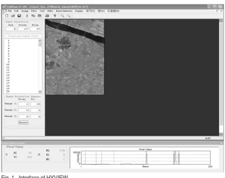
Fig. 1 shows the interface of HYVIEW where the hyperspectral image is displayed band by band to visualize the reflectance at the corresponding wavelength. In order to display as a color image, three bands are selected to play roles of red, green, and blue components. The selection can be made by typing the numbers of bands to the color component
Fig. 1. Interface of HYVIEW.
boxes or using one of the band selection utilities.
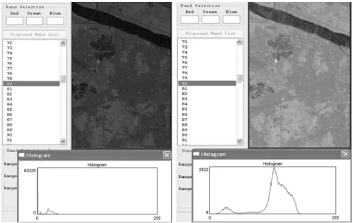
HYVIEW is able to display a hyperspectral image saved in the BIP format. Each band of the image is considered a grey scale image that can be viewed independently. To display an image as grey scale image, the pixel values should be scaled to be within a given dynamic range (usually 0 -255). In this program the log scaling is applied instead of linear scaling in order to be able to display effectively bands with a weak reflectance. This scaling can be equated as:
Y = log
2(X)*K (Eq. 1) K =
where X and Y are the pixel values before and after scaling, respectively, and K is a scaling constant;
max
Xand max
Yare in turn the maximum histogram bounds before and after scaling. Furthermore, in order to improve the display for each band, the scaling is done locally, that is, the values in the current displaying band are scaled independently to other bands. A comparison of these two scalings is illustrated in Fig. 2 where each scaling is applied on
the same band.
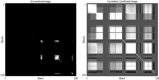
3) Displaying Correlative Quantities
For the aim of viewing the correlation among more than 200 spectral bands and supporting for further processing, the covariance and correlation coefficient matrices are computed and can be viewed as grey scale images. The mathematical definitions of above quantities used in hyperspectral data are given below:
C
z×z= {c
ij= (x[i]
mn_x[i] ___
)(x[j]
mn_x[j] ___
)}
(2) R
z×z= {r
ij= }, 1≤i, j≤z
where C, R are in turn the covariance and correlation coefficient matrices; w, h, z are 3 dimensions of the hyperspectral data (the number of columns, of rows and of bands, respectively); the bar denotes the mean value of each band; c
ij, r
ijare the covariance and the correlation coefficient between the ith and the jth bands, respectively. These symmetric images provide users with a visual display and useful information for choosing suitable bands to use. Fig. 3 shows these
c
ijc
iic
jjS
w n=1S
w m=1max
Ylog
2(max
X)
Fig. 2. A comparison between linear scaling (left) and log scaling (right) on the same band.
228 ×228 images corresponding to our hyperspectral data.
The above quantities are viewed using a linear scaling that maps the minimum values to 0 and the maximum values to 255. However, for avoiding the redundancy of the minus sign in these two images, the displayed image for covariance corresponds to the absolute value, where blacks indicate zero covariance and whites show the maximum absolute values. In this image, the large values focus on noisy bands where the reflective noises make the variances as well as the covariance between the bands prominent.
As for the correlation coefficient, values from -1 to 1 are linearly mapped, hence the blacks indicate -1’s;
the whites indicate 1’s and the grey tone represents near-zero value. Information extracted from these images may be useful for removing noisy bands from the original data.
4) Per-pixel view and Histogram
The plot at the bottom in Fig. 1 shows the per-pixel signal of raw reflectance value at a position in the image. Once the raw image data were atmospherically corrected, this plot can be a full reflectance curve. The position is updated as the
mouse pointer moves over the image. The X and Y indexes indicate the current position and the R, G, B values show the R, G, B components (color image).
The horizontal axis shows the number of bands; the vertical axis shows the intensity value range of the image. The vertical red line (or lines) indicates the current band (if viewing as grey-scale) (or 3 bands (if viewing as color image)).
The histogram is shown in accordance with the log scaling that is being used to display the hyperspectral data. Note that the data values used in calculation remain unchanged; the scaling is merely for display.
Fig. 3. Images of absolute covariance (left - after a contrast enhancement) and correlation coefficient (right).
Fig. 4. Per-pixel view in HYVIEW.
Fig. 5. Histogram of one band in HYVIEW.
Also, the analysis tool includes other image processing functions: zooming in/out, creating binary image by thresholding, converting, and vertically or horizontally flipping.
3. Processing functions
1) Band selections
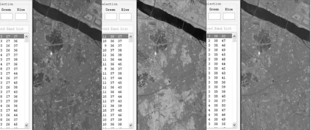
In order to view the image as a color image, 3 bands in the data are combined to create 3 composites of R, G, and B. In HYVIEW, three popular measures of optimal RGB band selection are chosen and implemented: the Optimum Index Factor OIF (Chavez et al., 1982), Sheffield Index SI (Sheffield, 1985) and Crippen Index CI (Beauchemin and Fung, 2001). The aim of band selection algorithms is to pick out 3 bands within the hyperspectral data that can provide the best visual appearance. Selecting bands for displaying in a color image is quite time consuming since many combinations have to be tried.
The OIF is a statistical approach to rank all possible 3-band combinations based on total variance within bands and correlation coefficient between bands. The calculation of this index is shown as follows:
OIF = (Eq. 3)
where s
iis the standard deviation of band i and r
ijis the value of the correlation coefficient between any two of the possible three pairs. Three-band combinations with high total variance within bands and low correlation coefficient between bands will have a high OIF. These combinations are expected to have the maximum extractable surface-type information since they use bands with the least redundancy in the remotely sensed data.
The second measure, Sheffield Index, considers the size of the hyperspace spanned by the data bands.
Sheffield suggests choosing bands with the biggest hypervolumes, since that selection would avoid band pairs having high correlation coefficients. The hypervolume can be approximated by the square root of the product of the eigenvalues associated with three principal components. As highly correlated image band pairs will have the eigenvalue of one of the two image bands close to zero, the hypervolume spanned by bands containing those pairs therefore will be small. The calculation of this measure is simplified by Eq. (4), since the product of eigenvalues is equal to the determinant of the covariance matrix.
SI = ΩCov
3×3Ω (Eq. 4) where Ω Ωdenotes the determinant and Cov
3×3indicates the 3×3 matrix extracted from the covariance matrix corresponding to positions of 3 considering bands. The three-band combination associated with the maximum value of determinants is selected.
The last measure, Crippen Index, can be considered a modified version of SI in which the individual band variance is removed in the ranking process, emphasizing on only the amount of correlation between band pairs. Referring to Anderson (1958) enables us to express the determinant of the covariance matrix as:
ΩCov
3×3Ω= s
is
js
k(1+2r
ijr
ikr
jk_r
2ij_r
2ij_r
2jk) (Eq. 5) When the value of r
2ijdecreases, the level of redundant information between the two bands decreases as well. The modification is done by dividing the SI by the product of individual band variances included in each combination. CI is defined as following:
CI = ΩCov
3×3Ω/ P
3s
i(Eq. 6)
i=1
s
iΩ r
ijΩ
S
3 i,j=1(i<j)S
3 i=1An example for illustrating these band selection algorithms is provided in Fig. 5 where the three algorithms are in turn applied to find the visually best 3-band combination of the first 50 bands from our data of 228 bands.
As aforethought, the difference in the criteria among the three selection schemes results in distinct band combinations, and the best combinations of one method may not appear in the tops of the others. The difference in the color tones does not mean a thing due to the assignment of bands as R, G or B composites. As analyzed by Beauchemin and Fung (2001) that the individual band variance in fact has no effect on the OIF index and as a result, the OIF and CI give combinations with a neutral color appearance. On the contrary, due to paying attention to this factor, the result of SI provides a better color contrast. For the runtime, the OIF demonstrates the fastest while SI and CI take almost the same amount of time inasmuch as the determinant calculation.
2) Atmospheric correction
Atmospheric correction of hyperspectral data is basically to remove atmospheric attenuations from the at-sensor radiance and to achieve surface
reflectance value, which can be analyzed with various sources of known spectral characteristics of surface materials (Griffine and Burke, 2003; Qu et al.,2003).
Eq. (7) is the basic equation for atmospheric correction. The surface reflectance value (r) is then calculated by the inversion of Eq. (7).
L(l) = L
p(l) + t(l)r(l)E
g(l)/p (Eq. 7) L(l): Sensor-received radiance for each channel l L
p(l): Path radiance
t(l): Atmospheric transmittance r(l): Surface reflectance E
g(l): Global flux on the ground
For inversion processing, path radiance, atmospheric transmittance, and radiation flux on the ground are obtained from the look-up-table, which were pre-calculated using the MODTRAN radiative transfer model with several input parameters of atmospheric and geometric conditions. The radiance value (L) can be easily obtained by applying the known calibration coefficients to pixel’s digital number of Hyperion data.
For fast and simple atmospheric correction of Hyperion data, HYVIEW uses pre-calculated LUT.
Detailed descriptions regarding the algorithms of atmospheric correction of hyperspectral data and the input parameters can be referred to Kim et al. (2007).
Fig. 6. A comparison of band selections on the first 50 bands: SI (left), OIF (middle) and CI (right).
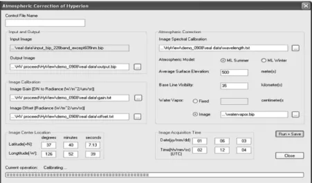
Fig. 7 shows the interface of atmospheric correction utility of HYVIEW. Users need to fill several input parameters including sensor characteristics, solar and sun geometry, and atmospheric information.
Atmospheric information is composed of the atmospheric model, surface elevation, visibility, and atmospheric water vapor content.
The reflectance image is saved in another file and can be displayed and used. There are two options of using atmospheric water vapor information to calculate the reflectance value: using a fixed water vapor value or loading a pre-calculated water vapor data. A water vapor file can be considered a water vapor image which has the same size as the hyperspectral image; each pixel contains the atmospheric water vapor content at the same position in the hyperspectral image. In this experiment, the size of the hyperspectral image was 400 (row)×256 (pixel)×228 (bands) and the runtime for atmospheric correction is less than 1 minute if using a fixed water vapor value and about 4 minutes if a water vapor image is loaded, evaluated on a computer CPU P4 2.8GB, 1GB memory. Fig. 8 shows spectral reflectance curves of several ground features extracted from the atmospherically corrected
Hyperion reflectance image. Although these spectra show some noise that may come from the Hyperion sensor itself, they acceptably agree with the typical form of spectral reflectance.
4. Conclusions and Future Works
This work is to provide an analysis tool for processing hyperspectral images from a collection of the state-of-the-art algorithms. In order to best display the hyperspectral images visually, the log
Fig. 7. Interface of atmospheric correction utility within HYVIEW.Fig. 8. Spectral reflectance curves of various targets extracted from atmospheric corrected Hyperion data (Kim et al., 2007).