Matlab을 이용한 해양파도 표면의 해석
응인요*․박수홍**
Analysis and Realization of Ocean Wave Surface by Utilizing Matlab
Ng Yin Yeo*․Soo-hong Park**
요 약
본 논문은 matlab을 개발툴로 사용하여 해양파도의 표면운동의 해석에 대한 것이다. 해양의 파도 및 바다 표면파에 대하여 이론에 근거하여 해석에 대하여 연구하였다. 또한 3차원 바다파도와 2차원 바다파도의 운 동을 Matlab을 이용하여 시뮬레이션하고 각각의 운동 형태를 시뮬레이션을 통하여 분석하고 그 결과를 고찰 하였다.
ABSTRACT
This research is about the studies of ocean wave and realization of ocean wave surface utilizing the Matlab as development tool. In this paper, the related background theory about ocean wave and sea-surface wave had been discussed. In addition, the three-dimensional and two-dimensional sea wave and sea-surface also been realized and simulated by using Matlab.
키워드
ocean wave, Matlab, wave spectrum , directional wave spectrum
* 동서대학교 메카트로닉스공학과([email protected]) ** 교신저자, 동서대학교 메카트로닉스공학과([email protected])
Ⅰ. Introduction
The study about ocean wave had started long time ago. The occurrence of ocean in the earth cause what we are here today. It is important for us to continue study about it although the interrelated task had started long time ago.
Ocean is a worth study field and it widely covered various field of knowledge. The correlated field including Biological, Chemical, Physics, Mat- hematic and also many of the latest technologies nowadays are interested with the ocean related research study.
The computer graphic designer always cracked their brain to simulate a real live ocean wave in the virtual world. To achieve a merely real live ocean wave, designers always need to go back to the mathematics formula and physics’ theorem that related with the sea surface.
This field of study may useful in many ways.
The visualization of sea surface can help developers to imagine the sea conditions and characteristic during handling their ocean related tasks. This paper included the discussion of the ocean related theory, mathematical expression and the method of implementation of ocean wave surface.
Ⅱ. Ocean Wave
In this section, a brief description about some basic theory and principle that lie beneath ocean wave will be illustrated. Ocean is part of the earth system. The activities involve with it is the mediating process in the atmosphere (the transfers of mass, momentum and energy through the sea surface) [2].
The wind generated wave of the sea surface is a stochastic event and consists of irregular collection of crests and troughs. The multiple type of forces act on the sea surface cause the multiple waves with different wave length, different amplitudes, out of phase, different wave periods, and propagates in different direction.
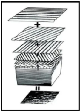
Fig. 1 The summation of all random cosine wave that form ocean wave. A concept drawing presented by
Pierson et al. 1955 [3].
Starting from a simple harmonic cosine wave, the wave propagating on a two-dimensional space which can represent by equation 1:
cos (1)
Where A is the amplitude, k=2π/λ is the wave-number,
is the wave-length, is the angular frequency, T is the wave period and is the phase of the wave. However, the ocean wave is the sum of all different sinusoidal waves.
cos (2)
Let us consider the ocean wave in two- dimension, a sum of cosine waves is one of the solutions that use to model the sea surface represented in equation 2.
Each of the cosine wave has its own amplitude, wave-number, angular frequency and phase. Figure 1 briefly illustrate the concept of ocean wave which form by sum of cosine wave, with each of them propagates with its own characteristic. Different locations also contribute to different type of wave.
As shown in figure 2, the wave at shallow water near the beach or river side and the wave in the deep water have two different patterns. The concern in this paper will more to the wave in the deep sea.
Fig. 2 The wave type occurs in shallow water and in deep water [5].
Ⅲ. Ocean Wave Spectra
To descript this complex ocean wave, the concept of ocean wave spectrum had been widely used. Previous section use the wave-length distribution and angular distribution to descript the ocean wave which shown in (2). To determine these distributions, physicists use the relationship of the wavelength and the frequency of the wave to perform ocean wave realization and analysis work.
There are several frequency distribution models that had been developed. The most famous and prominent models are Pierson Moskowitz model and
JONSWAP model. Following session will discuss more details about these models.
A. Pierson Moskowitz Spectrum
Various idealized spectra are used to answer the question in oceanography and ocean engineering.
Perhaps the most common and easiest is the one that proposed by Pierson and Moskowitz (1964) [2].
This spectrum model assumed the wind blew steadily for a long time over the wide sea area and thence the wave come into equilibrium with the wind. The formula for this energy distribution is shown in equation 3.
exp
(3)
The parameters for the formula are: α = 0.0081,
where v is wind velocity. fm is the peak frequency of the energy distribution or means the dominant wave type in the energy distribution for this frequency value.
Besides that, the dispersion equation had been used to determine the wavelength and the relationship of the wave number and frequency of the wave:
(4)
Where k is wave number, g is gravitational acceleration, and λ is wave length.
Figure 3 shows the Pierson-Moskowitz spectrum for five different wind speeds. The higher wind speed value, the higher for the wave energy distribution.
Fig. 3 The Pierson Moskowitz spectrum plotted using Matlab for five different wind speeds.
B. JONSWAP Spectrum
JONSWAP is the acronym for Joint North Sea Wave Observation Project. Base on the data collected from this project, Hasselmann et al.(1973) propose a modified version of Pierson Moskowitz spectrum. This modified version called JONSWAP spectrum. Its purpose is to account the wave limited fetch condition when he found out the wave spectrum is never fully develop during the JONSWAP project,
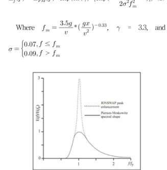
expln exp
(5)
Where
, = 3.3, and
≤ ≻
Fig. 4 The comparison of JONSWAP spectrum and Pierson-Moskowitz spectrum [7].
Ⅳ. ANGULAR DISTRIBUTION
Ocean waves are form by numerous random waves from all possible direction. Previously, we had discussed about the energy distribution of the wave, but it is yet not enough to represent the ocean wave. Ocean wave spectra should represent together with energy distribution and the angular distribution. The directional wave spectrum is written as equation below:
(6)
Next session will illustrate some common use angular distribution.
A. Mitsuyasu Angular Distribution Function Moreover, another commonly used angular distribution function in ocean wave realization is Mitsuyasu angular distribution function. This theorem is shown as below equation.
cos
(8)
∞ (9)
≥
(10)
The formula 8 describes the ocean wave propagation direction or in other words, it more precisely shows the energy of a wave with frequency, f that is travelling under the angle,
relative to the direction of the wind blow.
Ⅴ. IMPLEMENTATION AND RESULTS A. Realization of 2D Ocean Wave
The implementation started with generating the
Pierson Moskowitz spectrum and the Mitsuyasu angular spreading by applying the core (3) and (8).
As shown in figure 5, the bell shape of wave energy spectrum and two peak wave spreading pattern had been generated. Applying the equation 6, a directional wave spectrum had been generated.
From figure 6, graph b1, the wave spectrum now become a two peak spectrum due to it bounded with the angular spreading. A white noise had been generated in the process. The white noise technique is commonly using in ocean wave generation jobs.
This method is based on the principle of digitally filtered white noise and is generated in real time [8]. As shown in the figure 6, graph b2, the generated white noise spectrum is modulated with the directional wave spectrum. The directional wave spectrum which acts as the digital filter for the white noise that only allows a band-pass frequency for the noise spectrum.
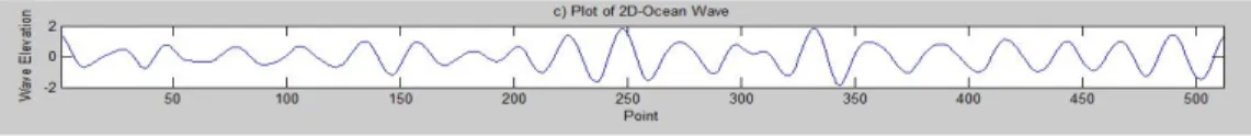
The final result had obtained by performing inverse FFT towards the filtered white noise spectrum. Figure 7 shows the generated 2D ocean wave with wind speed of 10m/s; while figure 8 shows the ocean wave with 30m/s wind speed. By comparing the wave magnitude in figure 7 and figure 8, we can conclude that higher wind speed will cause larger ocean wave. This also fulfills the theorem of Pierson-Moskowitz equation, which tells the wave in fully developed sea are rely on the magnitude of the wind.
B. Realization of 3D ocean wave
By applying the same algorithm and method, a 3D ocean wave realization may carry out straightforwardly. The difference between two tasks is it is more troublesome for 3D ocean wave when a three dimension ‘space’ need to ready for the process. By referring [9], the 3D dimension array being initialized.
After the initialization of the dimension, all the parameter needs to be setup as well. Next, a
Fig. 5 The Pierson Moskowitz spectrum in (a1) and the Mitsuyasu angular distribution in (a2).
Fig. 6 (b1) shows the Directional Wave Spectrum; (b2) shows the white noise filtered by the spectrum.
Fig. 7 The final output of two-dimensional ocean wave for wind speed 10m/s.
Fig. 8 The final output of two-dimensional ocean wave for wind speed 30m/s three-dimensional Pierson Moskowitz spectrum had
been generated. The following step is generating the 3D Misuyasu angular distribution. Therefore, a directional wave spectrum was created. The method continues and finally the directional wave spectrum transformed into the wave-number domain. The white noise method also applied in the 3D ocean wave realization. As same as previous work, the white noise spectrum modulated into the directional wave spectrum. At the end, the wave surface can be obtained by inverse FFT the modulated wave spectrum.
The following figures shows the steps mention above. Figure 10 shows the wave energy spectrum
and figure 11 shows the directional wave spectrum that used the Pierson-Moskowitz spectrum and Mitsuyasu spreading. Figure 12 shows the modulated spectrum in between the white noise spectrum and the directional wave spectrum, and this is the pre-final step of whole process.
From the figures, we can observe that the three dimensional spectrum output pattern is similar with the output pattern of the two-dimensional spectrum.
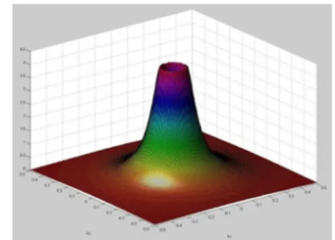
Lastly, the final result of the three-dimensional ocean wave was shown in figure 13.
Fig. 10 The 3D Pierson Moskowitz wave spectrum
Fig. 11 The directional wave spectrum.
Fig. 12 The modulated spectrum between white noise spectrum and the directional wave spectrum.
Fig. 13 The three-dimensional Ocean wave surface
Ⅵ. CONCLUSION AND FUTURE WORK
The ocean wave realization done in this research was base on the Pierson-Moskowitz spectrum and Mitsuyasu angular spreading concepts. Conse- quently, the output ocean wave characteristics are bounded by both theories. One of the most noticed characteristic for this work is it only applies for the fully developed ocean wave.
For future work, more type of wave energy spectrum will be applied with combine with multiple type of angular spreading method. Besides that, animating the ocean wave will be developing in future
REFERENCES
[1] Wikipedia, The free Encyclopedia. (2010). Wind Wave. Retrieved May 7, 2010, from http://en.wikipedia.org/wiki/Wind_wave [2] Robert H. Stewart, Introduction to Physical
Oceanography. Department of Oceanography, Texas A & M University, 2008.
[3] Danièle Hauser, Kimmo Kahma, Harald E.
Krogstad, Susanne Lehner, Jaak A. J. Monbaliu, Lucy R. Wyatt, Measuring and Analyzing the Directional Spectra of Ocean Waves. European cooperation in the field of scientific and technical research, COST, 2005.
[4] M.D. Earle, “Non-directional and directional wave data analysis procedures,” NDBC Technical Document 96-01. National Data Buoy Center (NDBC), Stennis Space Center, 1996.
[5] Dr. Heinz Seyringer. (2001). Nature Wizard.
Retrieved March 24, 2010, from http://www.naturewizard.com/
[6] Dr. Steven A. Hughes, “Directional Wave Spectra Using Cosine-Squared and Cosine 2S Spreading Functions,” Coastal Engineering Technical Note. Coastal Engineering Research Center, Coastal and hydraulics Laboratary, 1985.
[7] Dr. Andrew Laing, “Guide to Wave Analysis And Forecasting,” WMO-No. 702, second edition.
Secretariat of the World Meteorological Orga- nization, Geneva, Switzerland, 1998.
[8] HR Wallingford, “Long and short crested sea generation software for physical models,”
equipment datasheet.
[9] Orlando Rodríguez. (2009). Sea Surface.
Retrieved January 20, 2010, from
http://www.mathworks.com/matlabcentral/fileex change/24884-sea-surface/
저자 소개
응인요(Ng Yin Yeo) 1985년 7월 말레지아출생 2008년 말레지아 MMU졸업 (http:://www.mmu.edu.my)
현재 동서대학교 메카트로닉스공학과 석사과정
박수홍(soo-hong park) 1986년 2월 부산대학교 정밀기계 공학과 졸업 (공학사)
1989년 2월 부산대학교 대학원 기 계공학과 졸업(공학석사)
1993년 2월 부산대학교 대학원 기계공학과 졸업(공 학박사)
동서대학교 메카트로닉스공학과 교수
지식경제부, 국토해양부, 부산울산 건설기술평가위원, 중소기업청, 조달청 평가심의위원
※ 주 관심분야 : 제어 자동화, 로봇공학