접수일자 : 2010년 7월 7일 완료일자 : 2010년 10월 4일
*교신저자
A Hierarchical Clustering Method Based on SVM for Real-time Gas Mixture Classification
Guk-Hee Kim, Young-Wung Kim, Sang-Jin Lee and Gi Joon Jeon *
School of Electronics Engineering, College of IT Engineering Kyungpook National University
Abstract
In this work we address the use of support vector machine (SVM) in the multi-class gas classification system. The objective is to classify single gases and their mixture with a semiconductor-type electronic nose. The SVM has some typical multi-class classification models; One vs. One (OVO) and One vs. All (OVA). However, studies on those models show weaknesses on calculation time, decision time and the reject region. We propose a hierarchical clustering method (HCM) based on the SVM for real-time gas mixture classification. Experimental results show that the proposed method has better performance than the typical multi-class systems based on the SVM, and that the proposed method can classify single gases and their mixture easily and fast in the embedded system compared with BP-MLP and Fuzzy ARTMAP
.Key Words :
support vector machine, multi-class system, gas classification, hierarchical clustering method
1. Introduction
Over the past several years, we have studied a wire- less electronic nose network for monitoring real-time gas mixture, NH3 and H2S, main malodors in various environments[1][2]. The electronic nose system is com- posed of feature extraction, gas classification and gas concentration estimation. In the real-time quantitative analysis of gas mixtures, the gas classification process is very important step for better performance. Fuzzy ARTMAP and BP-MLP have been used for gas classi- fication and some encouraging results have been ach- ieved[3][4][5]. In spite of these achievements, some in- herent weaknesses, such as the multiple local minima problem, the choice of the number of hidden units, and the danger of over-fitting would make it difficult to put the networks into practice[6].
The SVM is a classification technique based on stat- istical learning theory. It is a powerful tool for data analysis with small sampling, nonlinearity and high dimension. The SVM has been successfully applied to classification tasks such as fault diagnosis [7] and face recognition [8]. But, because the use of the SVM in the field of signal classification has begun for binary class, the extension to the multi-class case is not straight- forward.
In this paper, we propose the HCM based on the SVM, where in the order of the average distance be-
tween the classes the layer of the SVM multi-class system is hierarchically determined. The proposed method is compared with BP-MLP and Fuzzy ARTMAP and has shown excellent performances. Also, it is compared with the results of the model of typical multi-class system based on the SVM. The results show that the proposed multi-class system has better performances than typical multi-class systems, OVO and OVA, on the training speed and reliability in the embedded system.
The rest of the paper is organized as follows: Section 2 introduces the SVM classifier. Section 3 presents the HCM based on the SVM for the multi-class system.
Section 4 explains a detailed experimental design.
Section 5 compares performances of the proposed model with other multi-class systems with the experimental data sets. Finally, Section 6 provides the conclusion.
2. Support vector machine
The SVM was developed based on the principle of structural risk minimization by Vapnik and co-workers [9]. Instead of minimizing error in the training data, the SVM minimizes a bound on the expected generalization error. The main idea of SVM classification is to find an optimal separating hyperplane by maximizing the mar- gin between the separating hyperplane and the data as shown in Figure 1. Two classes of sample points are represented by rings and squares, respectively. H is the optimal separating hyperplane, H1 and H2 are parallel to H and pass through the sample points closet to H.
The distance between H1 and H2 is defined as the
margin.
Given a set of training data T={
i
, yi
}, i=1,2,…,N, where
∊
denotes the input vectors, N is the number of training data and
∈{+1,-1} stands for the class label. When two classes are linearly separable and the margin is maximal, the hyperplane that sepa- rates the given data is determined by;Fig. 1. Separation of two classes by SVM.
(1)where ∈
denotes the weight vector and ∈
is the bias term. The separating hyperplane should satisfy the constraints
≥ ⋯
(2) When two classes are non-linealy separable, positive slack variables i
≥ is necessary to measure the vector i that lies on the wrong side of the margin.Then, the separating hyperplane should satisfy the fol- lowing inequality
≥
⋯
(3) Now, according to the principle of structural risk minimization, the optimal hyperplane separating the data can be obtained by optimizing the following objective function
minimize
║║
(4)subject to
≥
⋯
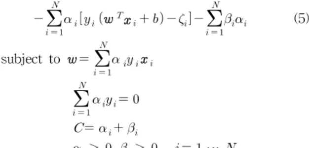
where the parameter C is defined as the trade off pa- rameter between the margin and the error.By applying the Lagrangian principle, the above opti- mization problem is transformed into the dual quadratic optimization problem as follows [10].
Maximize
∥∥
(5)subject to
≥
≥ ⋯
,Equation (5) can be expressed in a compact from [11]
Maximize
(6)Subject to
≤
≤
⋯
where ∈
is a Lagrangian multiplier. Then, the op- timal linear separating hyperplane is optained as follows. {
} (7)
In case of nonlinear problems, a nonlinear mapping function is employed to map the original input space
to N-dimensional feature space, where the nonlinear problems are possible to be classified as the linear problems. Then, the nonlinear classifier is {
} (8)where
is the kernel function. In the SVM, the commonly used kernel functions are as follows. The radial basis function;
║
║
(9) the polynomial basis function ;
(10) where d is an integer, and the sigmoid function;
(11) where p and v are positive constants.Parameter optimization becomes complex when using radial basis functions and sigmoid functions, since in radial functions the part below the decimal point of the parameters must be determined and sigmoid functions has two parameters to be optimized. Meanwhile, since in the polynomial basis functions for the SVM only one positive integer as a variable needs to be determined, the amount of the calculation time is small. Thus, in this work, the polynomial basis function is used in the SVM.
OVA
K
MK = MK
2OVO
K(K-1)/2
2M = MK(K-1)
HCM
K-1
M(K-n)= MK(K-1) -M(K-2)(K-1)/2
3. Hierarchical clustering method based on SVM for multi-class system
The SVM was originally developed to solve binary problems. To solve multi-class problems based on the SVM, different approaches-OVA and OVO which com- bine several two-class SVMs have been presented in [12]. Suppose we have K classes and samples for k-th class. In OVA strategy, K SVM models are needed.
The k-th SVM is trained with all training samples of the k-th class with positive labels, and the rest samples with negative labels. A test sample belongs to the class that has the largest value of the indicator function.
⋯
⋯
(12) where
and
are the weight vector and the bias term of k-th SVM, respectively.In the OVO strategy, K(K-1)/2 SVM models are de- signed, where each one is trained with input data of two classes. The i-j SVM with the weight vector and the bias term is trained with i-th class data as pos- itive labels and j-th class data as negative labels. To classify a test sample a voting system is needed. If the indicator function
implies that be- longs to i-th class, the vote for i-th class is increased by one, otherwise the vote for j-th class is increased by one. The test sample belongs to the class that has the largest value of the vote.Contrary to the OVA and OVO strategies, in the proposed HCM the layer of the SVM multi-class sys- tem is hierarchically determined in the order of the average distance between the classes. The first SVM is trained with training samples of the farthest class with positive labels, and the rest classes with negative labels. Next, the SVM in the second layer trained with the remaining samples except the samples trained as class1 in the first layer. Like the previous layer, the samples of the farthest class have positive labels, and the rest classes have negative labels. In this way, all SVM layers can be constructed as shown in Figure 2.
Fig. 2. Multi-class system classified by the HCM.
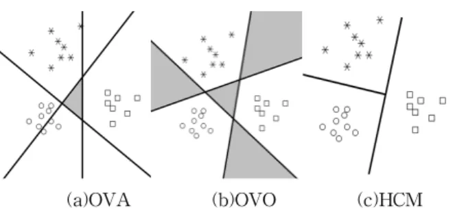
Compared with OVA and OVO, the proposed mul- ti-class system is very simple and fast because it has the smallest total number of training as shown in Table 1. Sometimes, although OVO improves the results, it is not the best for real time gas classification because even in the case where the number of data is small, the number of SVM classifiers increases. Moreover, both OVA and OVO have disadvantage of rejection area which can be seen as shadow areas in Figure 3. In the rejection area, the test samples cannot be classified to any classes. Notice that the proposed HCM has no re- jection area.
Table 1. The number of SVM classifiers and the total number of training of OVA, OVO and the proposed method*
*M is the average number of data per class and K is the number of classes
(a)OVA (b)OVO (c)HCM Fig. 3. Possible rejection areas of OVA, OVO and the
proposed method for three classes
4. Experimental design
Fig. 4. Structure of gas classification system To classify the gases and their mixture, the system is composed of data extraction, preprocessing, learning, and
testing. Details on these steps are shown in Figure 4.
4.1. Experiment and data acquisition
Ammonia and hydrogen sulfide were chosen as target gases, and experimental system for the data acquisition was prepared with the following three parts–gas lines, a bubbler and a test chamber (Figure 5). The gas lines are composed of four gas bottles which contain NH3, H2S and dry synthetic air (nitrogen: oxygen=4:1) and four mass flow controllers (MFCs). The synthetic air line is connected to the bubbler and then intermixed with the target gas via gas lines. The experiment was conducted under the following conditions. The temper- ature of experimental glass chamber was maintained at 27°C with 52% humidity. The total flow rates of the MFCs were set at 278cc/min, and the chamber capacity was 2250cc.
Fig. 5. Experimental design for data acquisition
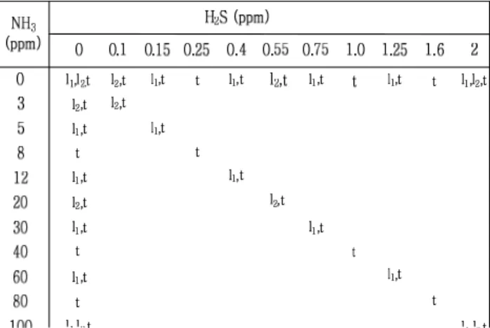
Table 2. Concentration compositions of the target gases*
*The concentration for training subset 1 is marked by ‘l
1’, subset 2 by ‘l
2’, and test set by ‘t’
Measurements of the target gases H2S, NH3, and mixture of the two gases were carried out at 30 differ- ent concentrations as shown in Table 2. The concen- tration of each gas is measured after stabilizing gas chamber by injecting the reference air. The gas with the chosen concentration is injected through MFCs and is saturated in the chamber, then, 30 experimental data are obtained. In this way, eleven measurement cycle s
including reference air for each gases–NH3, H2S, and mixtures were carried out.
One data sequence composes the sensor heater turn on period for 6s and turn off for 6s repeatedly, reading the output voltage changes of the SnO2-CuO and SnO2-Pt sensing films for 1.425㎲ with 57㎳ interval, resulting in a 50-dimension data set extracted from the two sensing films. The extracted data set are trans- mitted from slave sensor node to master sensor node via an RF transceiver and then, the master sensor node sends the received data to the host computer through a USB interface. For details, see the reference [2]. From these 50–dimension data set a 6-dimension data set was extracted by the variable selection technique [13].
4.2. SVM for electronic nose system
Based on the extracted features, three SVMs are de- veloped to classify the four gas types: air, NH3, H2S, and the mixture. Firstly, in the order of their average distance of air, NH3, H2S, and the mixture, the layer of the hierarchical SVM multi-class system is determined.
Then, training samples can train the SVM by clustering results. With all training samples, the first SVM is trained to separate air from other three gases. With the samples of other three gases, the second SVM is trained to separate NH3 from the other two gases. With the samples of other two gases, the third SVM is trained to separate H2S from the mixture gas. The total 270 samples for subset 1 : 45 air samples, each 15 samples at 15 different concentration levels and the to- tal 180 samples for subset 2 : 45 air samples, each 15 samples at 9 different concentration levels were used in the training of the proposed system as shown in Table 2. The polynomial basis functions with d = 2 and 3 are chosen as kernel functions.
To classify unknown test samples by the proposed multi-class system, a test sample is fed to the first SVM. If the output of the first SVM is 1, the test sam- ple is classified as air and the gas recognition is finished. If the output of first SVM is –1, the second SVM accepts the test sample as the input. If the output of the second SVM is 1, the test sample is classified as NH3, and the gas recognition is finished. If output data of the second SVM is –1, then the test sample is fed to the third SVM. If the output of the third SVM is 1, the test sample is classified as H2S. If the output of the third SVM is –1, the test sample is classified as the mixture gas. Total of 495 samples: 45 air samples, each 15 samples at 30 different concentration levels for sin- gle gases and the mixture have been classified in this manner.
5. Results and Discussion
The experimental results of the proposed model are compared with the results of the other models of typical
Kernel function
Value of C
parameter OVA OVO HCM
poly(2)
1 77.78 78.79 87.88
10 82.63 96.57 96.57
100 91.92 98.79 98.79
1000 98.39 100 100
10000 98.59 100 100
poly(3)
1 75.76 84.85 90.91
10 82.83 96.77 98.57
100 91.92 99.60 98.79
1000 96.97 100 100
10000 98.59 100 100
Kernel function
Value of C
parameter OVA OVO HCM
poly(2)
1 84.04 75.76 72.53
10 81.82 93.94 93.94
100 90.79 98.38 98.38
1000 90.79 97.98 97.98
10000 90.79 97.98 97.98
poly(3)
1 71.11 85.05 87.48
10 90.91 96.97 96.97
100 86.87 97.17 97.17
1000 85.86 97.17 97.17
10000 86.26 97.17 97.17
Method
Fuzzy ARTMA
P
BP_ML
P HCM
Subset1
Network
size 6/16(I/O) 6/18/4
(I/H/O) N/A
Iterations 3 10000 N/A
Parameter ρ = 0.956
α = 0.01 η = 0.5
d = 2 C
=1000 Classificat
ion rate 88 100 100
Subset2
Network
size 6/7(I/O) 6/18/4
(I/H/O) N/A
Iterations 3 10000 N/A
Parameter ρ = 356
α = 0.01 η=0.5
d = 2 C =
100 Classificat
ion rate 84.44 94.54 98.38
SVM multi-class in Table 3 and Table 4. In the em- bedded system, it is required that the amount of calcu- lation time is small and the parameter optimization is simple. Therefore, polynomial basis functions with de- grees (d) 2 and 3 are used as the SVM kernel functions and they are denoted by poly(2) and poly(3) in Tables 3 and 4. The optimal regulation parameter C is selected by the user. In each experiment, to find the optimized parameters, ‘d’ and ‘C’ we trained with the parameters in various range and tested with the samples as shown in Table 3 and Table 4. The adjusted parameters with maximal classification accuracy can be selected as the most appropriate parameters in the embedded system.
By the simulation results with the real data, the OVA method has shown relatively worse performance than the other methods and different results on different parameter of ‘C’. By contrast, the OVO method and the method we proposed have similar performance with pa- rameter ‘C’ of almost all range. Also, in the real em- bedded system considered must be not only the accu- racy rate but the capacity and speed. Compared with the OVO method that has 6 SVM classifiers, the sug- gested model with 3 SVM classifiers is simple and fast.
Therefore, all things considered, it can be noticed that the proposed multi-class system has advantages over other multi-class systems based on the SVM.
Table 3. Classification rates of multi-class systems based on SVM for subset 1
Table 4. Classification rates of multi-class systems based on SVM for subset 2
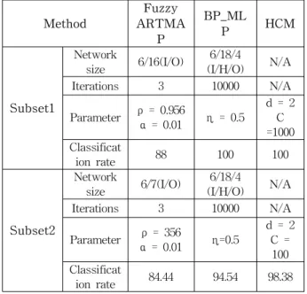
Table 5. Comparison of classification rates with other classification methods
In order to compare the classification rate of the pro- posed multi-class system with BP-MLP and Fuzzy ARTMAP, the proposed multi-class system with the optimized parameters d = 2 and C = 1000, Fuzzy ARTMAP with network size 6/16 (input/output) layers and the optimized vigilance parameter ρ = 0.956, the choice parameter α = 0.01 and BP-MLP with network size 6/18/4 (input/hidden/output) layers and the learning parameter η = 0.5 are trained with the same training samples for subset 1 and tested in the embedded system. The same classification test has been applied to the subset 2 with slightly different parameters and the test results are shown in Table 5. Compared with BP-MLP and Fuzzy ARTMAP, the proposed mul- ti-class system has shown the best performance on the classification rate for both subset 1 and subset 2.
6. Conclusions
In this paper, a hierarchical clustering method based on the SVM is designed and applied to the problem of gas classification. The simulation results with the real data show that the proposed multi-class system has not only high classification rate but small calculation time.
Thus, all things considered, in gas mixture classification the proposed method has the best performance among multi-class systems based on the SVM. Also, in the embedded system, the experimental results of the em- bedded system show that the proposed multi-class sys-
tem has better performance than BP-MLP and Fuzzy ARTMAP on the classification rate.
References
[1] J. H. Cho, Y. W. Kim, K. J. Na, and G. J. Jeon,
"Wireless electronic nose system for real-time quantitative analysis of gas mixtures using mi- cro-gas sensor array and neuro-fuzzy network,"
Sens. Actuators B, vol. 134, pp. 104-111, 2008.
[2] Y. W. Kim, S. J. Lee, G. H. Kim, and G. J. Jeon,
“Wireless electronic nose network for real-time gas monitoring system,” Proc. of the 2009 IEEE
International Workshop on Robotic and Sensors Environments, pp. 169-172, Nov. 2009.
[3] E. Llobet, E. L. Hines, J. W. Gardner, P. N.
Bartlett, and T. T. Mottram, “Fuzzy ARTMAP based electronic nose data analysis,”
Sens.
Actuators B, vol. 61, pp. 183-190, Dec. 1999.
[4] A. Gulbag, and F. Temurtas, “An intelligent gas concentration estimation system using neural network implemented microcontroller,”
Lect.
Notes Comput. Sci., vol. 3339, pp. 1206-1212,
Nov. 2004.[5] A. Gulbag, and F. Temurtas, “A study on quan- titative classification of binary gas mixture us- ing neural networks and adaptive neuro-fuzzy inference system,” Sens. Actuators B, vol. 115, pp. 252-262, May 2006.
[6] X. D. Wang, H. R . Zhang, and C. J. Zhang,
“Signals recognition nose based on Support vector machines,” Proc. of the 2005 IEEE the Fourth
International Conference on Machine Learning and Cybernetics, pp. 3394-3398, Aug. 2005.
[7] S. Jiang, W. Gui, C. Yang, and Y. Xie, “Fault Diagnosis of Lead-Zinc Smelting Furnace based on Multi-Class Support Vector Machines,” Proc.
of the 2007 IEEE International Conference on Control and Automation, pp. 1643-1648, June, 2007.
[8] J. W. Lu, K. N. Plataniotis, and A. N.
Venetsanopoulos, “Face recognition using feature optimization and support vector learning. Neural Networks for Signal Processing XI,” Proc. of the
2001 IEEE Signal Processing Society Workshop,
pp. 373-382, Sep. 2001.[9] V. N. Vapnik, The Nature of Statistical Learnig
Theory, John Wiley & Sons Inc., NewYork, 1999.
[10] C. Distante, N. Ancona, and P. Siciliano,
“Support vector machines for olfactory signals recognition”, Sens. Actuators B, vol. 88, pp.
30-39, 2003.
[11] I. S. Oh, Pattern Recognition ,Kyobo Book Co., 2008.(in Korean)
[12] C. W. Hsu, C. J. Lin, “A comparison of methods for multi-class support machines,” IEEE Trans.
Neural Net., vol. 13, pp. 415-425, 2002
[13] J. Berezmes, P. Cabre, S. Rojo, E. Llobet, and X.
Correig, “Discrimination between diffefent sam- ples of olive oil using variable selection techni- ques and modified fuzzy ARTMAP neural net- works,” IEEE Sens. J., vol. 5, pp. 463-470, 2005.
저 자 소 개
Guk-Hee Kim received the B.S.
degree in Electronics Engineering from Kyungpook National University, Daegu, Korea in 2009. Since 2009, she has studied for a master's degree in Kyungpook National University. Her main research interests are currently pattern recognition and sensor signal processing.
Young-Wung Kim received the B.S.
degree in Electronics Engineering from Kyungil University, Gyeoungsan-si, Gyeongsangbuk-do, Korea in 2006. He received the M.S. Degrees in Electronics Engineering from Kyungpook National University in 2008. Since 2008, he has studied for a doctor's degree in Kyungpook National University. Her main research interests are currently embedded system, sensor network and electronic olfactory system.
Sang-Jin Lee received the B.S. degree in Electronics Engineering from Yeungnam University, Gyeoungsan-si, Gyeongsangbuk
-do, Korea in 2009. Since 2009, he has studied for a master's degree in Kyungpook National University. His main research interests are currently sensor drift and environmental monitoring system.
Gi Joon Jeon received the B.S. degree in Engineering from Seoul National University, Seoul, Korea in 1969. He received the M.S. and Ph.D. Degrees in Systems Science and Engineering from University of Houston, Houston, TX in 1978 and 1983, respectively. Since 1983, he has been with the School of Electronics Engineering, Kyungpook National University. His main research interests are currently intelligent control and sensor signal processing.