Bayesian pooling for contingency tables from small areas

Bayesian pooling for contingency tables from small areas

Aejung Jo ¹ · Dal Ho Kim ²

12 Department of Statistics, Kyungpook National University

Received 18 September 2016, revised 13 October 2016, accepted 24 October 2016

Abstract

This paper studies Bayesian pooling for analysis of categorical data from small ar- eas. Many surveys consist of categorical data collected on a contingency table in each area. Statistical inference for small areas requires considerable care because the subpop- ulation sample sizes are usually very small. Typically we use the hierarchical Bayesian model for pooling subpopulation data. However, the customary hierarchical Bayesian models may specify more exchangeability than warranted. We, therefore, investigate the effects of pooling in hierarchical Bayesian modeling for the contingency table from small areas. In specific, this paper focuses on the methods of direct or indirect pool- ing of categorical data collected on a contingency table in each area through Dirichlet priors. We compare the pooling effects of hierarchical Bayesian models by fitting the simulated data. The analysis is carried out using Markov chain Monte Carlo methods.

Keywords: Contingency table, Dirichlet prior, hierarchical Bayesian, Markov chain Monte Carlo, pooling, small areas.

1. Introduction

In many surveys, the sample data consist of the categorical variables collected on a contin- gency table in each small area. The analysis is performed in subpopulations corresponding to small areas as well as whole population. We should take care of a precision which is affected by the sample size in small area estimation. One way to resolve a precision problem is to borrow the information from the neighboring areas via the hierarchical model. That is, we can consider the pooling strategies for borrowing strength in small areas.

There has been a continuously increased interest in methods for pooling of data. Espe- cially, Malec and Sedransk (1992) developed a Bayesian procedure for estimation of the means for the specified experiments among a set of seemingly similar experiments. They constructed the prior distribution for location parameter to reflect the their assumptions.

There are subsets of parameters such that the parameters with subscript for each subset are very similar, and there are uncertainty about the composition of subsets of parameters.

They specify the prior distribution for parameter through conditioning on same subscript in similar experiments. The proposed flexible prior distribution allows the intensity and nature

1 Ph.D. candidate, Department of Statistics, Kyungpook National University, Daegu 41566, Korea.

2 Corresponding author: Professor, Department of Statistics, Kyungpook National University, Daegu

41566, Korea. E-mail: [email protected]

of the pooling to be influenced by the sample data. After, Evans and Sedransk (1999) pro- posed an alternative Bayesian model with covariates that is more flexible. And Evans and Sedransk (2003) provided a fully Bayesian justification for the results in Malec and Sedransk.

In above three papers, their models have been extended with the same key concept which is specified in the model using the same subscript in similar experiments. Recently Donson (2009) developed methods for Bayesian nonparametric modeling of multivariate categori- cal data using Dirichlet process mixtures of product multinomial models which allow local pooling.

In this paper, we construct the hierarchical Bayesian pooling models with the Dirichlet distributions as the prior distributions. The interested parameters are indirectly allowed a borrowing strength from neighboring areas through the hyperparameters of the Dirichlet distribution. In the other words, the common effect of responses about the total areas is re- flected from the hyperparameters, while the detail fluctuations comes through a hierarchical structure of the Bayesian model in each area. To investigate the pooling effects in hierarchi- cal models, we consider the simulated contingency table which consists of categorical data in the area. Recently Bayesian small area models in the contingency tables with nonresponses have been studied in Woo and Kim (2015, 2016).

The outline of the remaining sections is as follows. In Section 2, we introduce hierarchical Bayesian pooling models for the analysis of categorical data from small areas. In Section 3, we study Bayesian inferences using the Markov chain Monte Carlo (MCMC) method. We compare the results of numerical study in Section 4. Then we give our concluding remarks in Section 5.

2. Model specification

We consider the I × K contingency table with cell count n ik which is a kth response in ith areas, i = 1, · · · , I, k = 1, · · · , K. Let π ik denote the corresponding probability of each unit cell. We assume that

n i |π i

iid ∼ Multinominal(n i , π i ) (2.1) where n i = (n i1 , · · · , n iK ) is the response vector, n i = P K

k=1 n ik is total sum of responses, and π i = (π i1 , · · · , π iK ) is the corresponding probability vector in ith area.

In the basic model (2.1), we assume that the parameter π i ’s are composed of various cluster. But we don’t know the cluster indicator for each π i through the information from sample data only. Therefore we focus on the Bayesian inference of the parameters and their cluster indicators at the same time. Our Bayesian pooling models are classified as the three types according to priors for π i for i = 1, · · · , I. The three types of pooling models are as follow:

1) No pooling π _i ^iid ∼ Dirichlet(1);

2) Complete pooling π ∼ Dirichlet(1) with π 1 = · · · = π I = π;

3) Adaptive pooling π i

iid ∼ Dirichlet(µτ ), where µ = (µ ₁ , ..., µ _K ), 0 ≤ µ _k ≤ 1, P K

k=1 µ _k = 1 and τ > 0 are hyperparameters

for Dirichlet distribution and are assumed to have the noninformative and proper prior

π(µ, τ ) = (K − 1)!/(1 + τ ) ² . This prior is very similar to a half-Cauchy prior and can pre- vent overestimation of scale parameters from our models. Recall that x|µ, τ ∼ Dirichlet(µτ ) has the density f (x|µ, τ ) = Q k

i=1 x ^µ _i

^{τ −1} /D(µτ ), 0 < x _i < 1, P k

i=1 x _i = 1 where D(µτ ) = Q k

i=1 Γ(µ i τ )/Γ(τ ), 0 < µ i < 1, τ > 0, is the Dirichlet function, also known as the multivari- ate Beta function.

In model 1, we assume that the data are not absolutely pooling. In other words, the areas are mutually independent and each π i for i = 1, · · · , I is concerned through each area’s data only. Therefore, the Bayesian inference may be affected by data because the prior distribution of π i is noninformative uniform Dirichlet distribution with parameter vector 1. Instead, the model 2 is just the opposite. We assume that the entire data are completely pooled. We can estimate one parameter using the entire data set. For the inference in complete pooling model, the several separated areas are constructed as one grand area. And it can improve the precisions since it allows a borrowing strength from all neighboring areas. On the other hand, the model 3 constructs the hierarchical structure for the parameters. The first stage of model 3 is not made by regional pooling. But, the pooling of data can be constructed second stage of the model using the hyperparameter µ and τ . Entire data share the same fixed effect, µτ , and the variation of parameters is dependent on the specific data in each areas.

3. Bayesian inference

Let n = (n ₁ , · · · , n _I ) be the response matrix and π = (π ₁ , · · · , π _I ) be the proportion parameter matrix for the model (2.1). And let Ω i = (π i , µ, τ ) be the parameter space corresponding to the ith area with π i , µ, and τ . Actually, the model 1 and 2 are a special case of model 3 which is an adaptive pooling model with parameters µ and τ . That is, the Bayesian inference for previous two models is deployed as model 3. In model 3, the joint posterior density of the parameters given data is obtained in the usual way by combining the likelihood and the prior distribution as follows.

π(Ω|n) ∝ n Y ^I

i=1

f (n|π _i )π(π _i ) o π(µ, τ )

∝

I

Y

i=1

n n i ! Q I

l=1 n lk !

K

Y

k=1

π _ik ⁿ

1 D(µτ )

K

Y

k=1

π ^µ _ik

^{τ −1} o (K − 1)!

(τ + 1) ²

∝

I

Y

i=1

n 1

D(µτ )

K

Y

k=1

π _ik ⁿ

^+µ

^{τ −1} o (K − 1)!

(τ + 1) ² (3.1)

where Ω = Ω ₁ × Ω ₂ × · · · × Ω _I , D(µ, τ ) = Q K

k=1 Γ(µ _k τ )/Γ( P K

k=1 µ _k τ ), µ = (µ ₁ , ..., µ _K ), 0 ≤ µ k ≤ 1, P K

k=1 µ k = 1 and τ > 0.

To run the Gibbs sampler, we draw numerical values in the followings.

(a) Full conditional for π i , i = 1, ..., I: Draw

π i |n i , µ, τ ∼ Dirichlet(n i + µτ ). (3.2)

(b) Full conditional for µ: Draw

π(µ|n, π, τ ) ∝

I

Y

i=1

n Γ( P K k=1 µ k τ ) Q K

k=1 Γ(µ k τ )

K

Y

k=1

π _ik ^µ

^{τ −1} o

(3.3)

where µ = (µ ₁ , · · · , µ _K ), P K

k=1 µ _k = 1, and 0 ≤ µ _k ≤ 1, k = 1, · · · , K. Let µ _(k) denote the vector of parameters except the kth component µ _k . Then we can obtain the conditional posterior density of µ _k given µ _(k) in each stage. In fact, we must have to estimate the K − 1 components of parameter, µ, sequentially. Then automatically calculate the Kth component value of µ using µ K = 1 − P K−1

k=1 µ k . Using the conditional posterior density (3.3), we can draw µ k , k = 1, · · · , K − 1 by grid method with support (0, 1 − P K−1

k

=1,k

6=k µ k

).

(c) Full conditional for τ : Draw

π(τ |n, π, µ) ∝

I

Y

i=1

nΓ( P K k=1 µ _k τ ) Q K

k=1 Γ(µ _k τ )

K

Y

k=1

π _ik ^µ

^{τ −1} o 1

(τ + 1) ² (3.4)

where τ > 0. We can use the grid method for τ also. Because the grid method can be used at closed support, we transform τ to ρ = 1/(1 + τ ), 0 < ρ < 1. Additionally, the Jacobian is 1/ρ ² . Then conditional posterior density of ρ can be written as follow.

π(ρ|n, π, µ) ∝

I

Y

i=1

n Γ( P K

k=1 µ _k ^1−ρ _ρ ) Q K

k=1 Γ(µ _k ^1−ρ _ρ )

K

Y

k=1

π ^µ

1−ρ ρ

−1 ik

o . (3.5)

4. Numerical study

We applied the hierarchical Bayesian pooling models to analyze the simulated data set.

Our analysis was done based on the contingency tables with cell count for 3 category in 20 areas. First, we generate the finite populations of size N = 100 from Multinomial distribution with probability π = (0.3, 0.2, 0.5) for 20 areas. Then the samples of size n = 20 are taken from this finite population. We calculated the finite population proportion for simulated data distribution in each areas using hierarchical Bayesian models with pooling structure.

Our finite population proportion is estimated by taking unseen part from Multinomial with estimating parameter π _i , i = 1, · · · , I (= 20) at each MCMC iterate. In detail, let N _ik for k = 1, 2, 3 be the total number of each level in ith area, but the value is unknown. On the other hand, we know the value n _ik for the seen part in data. Then we compute the finite population proportion (P _ik ) for i = 1, · · · , I using

P ik = 1 N _i

n

n ik + (N ik − n ik ) o

, k = 1, 2, 3 (4.1)

where N i − n i is unseen part responding from Multinomial distribution with parameter ˆ π i

which is estimated by our MCMC in each model. Then the posterior means and standard

deviations of the P _ik are obtained by the estimated empirical distribution of the P _ik . We

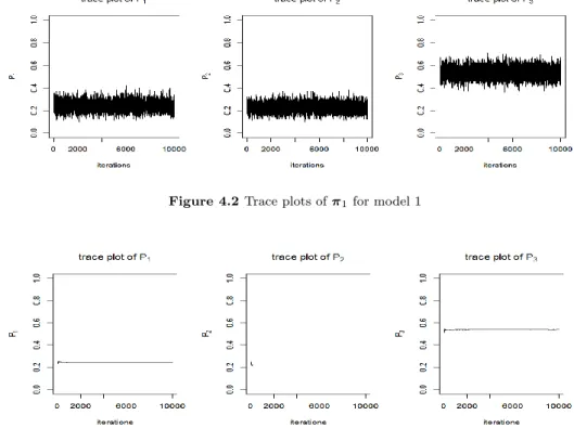
use 5000 iterates to burn out the MCMC and take every 10th estimated value to obtain 500

iterates.

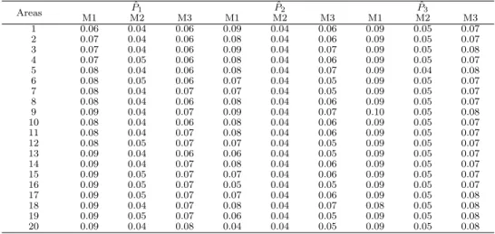
In Table 4.1 and Table 4.2, we report the posterior mean and standard deviation of finite population proportion from the three parametric models in 20 areas. A small posterior standard deviation is first evidence of good performance of hierachical Bayesian pooling models. The model 1 and 2 are the most extreme structures showing the influence of pooling for the data. Of course, the posterior standard deviations for the model with complete pooling are smaller than the model with no pooling since the data are used for only one parameter by complete pooling structure. In the model 2, the interested parameters have a uninformative prior, that is, uniform Dirichlet distribution. To provide the information of additional prior, we used to build the model 3. In the adaptive pooling model, we have incorporated the fixed effects based on data into the model. The fixed effect is indirectly estimated from entire data in adaptive pooling model.

Table 4.1 Posterior means for the finite population proportion (P 1 , P 2 , P 3 ) in simulated data with P = (0.2, 0.3, 0.5)

Areas P ˆ 1 P ˆ 2 P ˆ 3

M1 M2 M3 M1 M2 M3 M1 M2 M3

1 0.12 0.26 0.18 0.30 0.23 0.25 0.58 0.51 0.57

2 0.17 0.27 0.21 0.22 0.22 0.19 0.61 0.52 0.60

3 0.17 0.27 0.21 0.39 0.25 0.30 0.44 0.48 0.49

4 0.21 0.27 0.24 0.31 0.23 0.24 0.48 0.49 0.52

5 0.22 0.28 0.23 0.30 0.23 0.24 0.48 0.49 0.52

6 0.21 0.28 0.23 0.13 0.19 0.14 0.67 0.53 0.63

7 0.21 0.28 0.24 0.17 0.20 0.17 0.62 0.52 0.59

8 0.26 0.29 0.26 0.26 0.22 0.22 0.48 0.49 0.52

9 0.26 0.29 0.26 0.34 0.24 0.27 0.40 0.47 0.47

10 0.26 0.29 0.26 0.21 0.21 0.18 0.53 0.50 0.55

11 0.31 0.30 0.29 0.22 0.21 0.19 0.48 0.49 0.52

12 0.31 0.30 0.28 0.17 0.20 0.17 0.53 0.50 0.55

13 0.35 0.31 0.31 0.12 0.19 0.14 0.53 0.50 0.55

14 0.35 0.31 0.31 0.21 0.21 0.19 0.43 0.48 0.50

15 0.39 0.32 0.34 0.17 0.20 0.17 0.44 0.48 0.49

16 0.39 0.32 0.34 0.08 0.18 0.11 0.53 0.50 0.55

17 0.39 0.32 0.34 0.17 0.20 0.17 0.44 0.48 0.50

18 0.40 0.32 0.34 0.29 0.23 0.24 0.31 0.45 0.42

19 0.43 0.33 0.37 0.13 0.19 0.14 0.44 0.48 0.50

20 0.52 0.35 0.41 0.04 0.17 0.09 0.44 0.48 0.50

Table 4.2 Posterior standard deviations for the finite population proportion (P 1 , P 2 , P 3 ) in simulated data with P = (0.2, 0.3, 0.5)

Areas P ˆ 1 P ˆ 2 P ˆ 3

M1 M2 M3 M1 M2 M3 M1 M2 M3

1 0.06 0.04 0.06 0.09 0.04 0.06 0.09 0.05 0.07

2 0.07 0.04 0.06 0.08 0.04 0.06 0.09 0.05 0.07

3 0.07 0.04 0.06 0.09 0.04 0.07 0.09 0.05 0.08

4 0.07 0.05 0.06 0.08 0.04 0.06 0.09 0.05 0.07

5 0.08 0.04 0.06 0.08 0.04 0.07 0.09 0.04 0.08

6 0.08 0.05 0.06 0.07 0.04 0.05 0.09 0.05 0.07

7 0.08 0.04 0.07 0.07 0.04 0.05 0.09 0.05 0.07

8 0.08 0.04 0.06 0.08 0.04 0.06 0.09 0.05 0.07

9 0.09 0.04 0.07 0.09 0.04 0.07 0.10 0.05 0.08

10 0.08 0.04 0.06 0.08 0.04 0.06 0.09 0.05 0.07

11 0.08 0.04 0.07 0.08 0.04 0.06 0.09 0.05 0.07

12 0.08 0.05 0.07 0.07 0.04 0.05 0.09 0.05 0.07

13 0.09 0.04 0.06 0.06 0.04 0.05 0.09 0.05 0.07

14 0.09 0.04 0.07 0.08 0.04 0.06 0.09 0.05 0.07

15 0.09 0.05 0.07 0.07 0.04 0.06 0.09 0.05 0.07

16 0.09 0.05 0.07 0.05 0.04 0.05 0.09 0.05 0.07

17 0.09 0.05 0.07 0.07 0.04 0.06 0.09 0.05 0.08

18 0.09 0.04 0.07 0.08 0.04 0.07 0.08 0.05 0.08

19 0.09 0.05 0.07 0.06 0.04 0.05 0.09 0.05 0.08

20 0.09 0.04 0.08 0.04 0.04 0.05 0.09 0.05 0.08

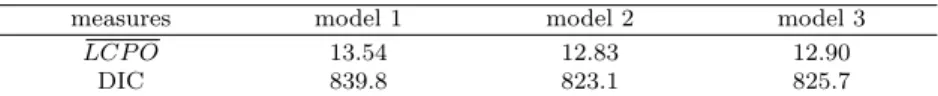
For the comparison of models, we will calculate the two measures to compare the perfor- mance each models. First, we calculate the deviance information criterion (DIC) which is a typical Bayesian model choice criterion to compare with the hierarchical Bayesian models.

Second, we calculate the logarithmic conditional predictive ordinate (LCPO) for evaluating the three model performance, which is a comparison method using a cross validation. For convenience of computation, we calculated the average of LCPO proposed by Gneiting and Raftery (2007) as follows.

LCP O = − 1 I

I

X

i=1

log(\ CP O _i ) (4.2)

where \ CP O i = P H

h=1 w h P (Y = y | Ω ^(h) ) for i = 1, · · · , I, w h =

P

h=1

f (Y =y| Ω

)

f (Y =y| Ω

) , P (Y = y | Ω ^(h) ) is likelihood of a single observation given parameter Ω ^(h) , and h = 1, · · · , H denote the iterates from the MCMC result under the hierachical Bayesian pooling model.

The average of LCPO measures the predictive ability of the models. The lower values of the mean of LCPO appear a better performance of the models.

Table 4.3 Comparison of DIC and LCPO under three different models

measures model 1 model 2 model 3

LCP O 13.54 12.83 12.90

DIC 839.8 823.1 825.7

As a result for MCMC, we have calculated the two measures to compare the models. In Table 4.3, we can show the value of two measures for each hierarchical Bayesian pooling model. Although the model 3 is more complicated than other two models, the performance is shown the similar value with model 2 which has the only one parameter for all areas.

It means the performance of model 3 with adaptive pooling effect is a pretty good for our simulated data although the dimension of parameter space is the biggest.

The posterior densities of three models are shown in Figure 4.1. The density of model 1 is probably more spread out than other models. The case of model 2 has a better precision than model 1, but the difference from true parameter value is larger. In model 3, the density of posterior has a distinct advantage over most other models. According to the indirect pooling effect, we can increase the precision of our model and decrease the bias from true value.

2 3

Figure 4.1 Comparison of densities under three different prior specifications

We have monitored the convergence of the Gibbs sampler using trace plots, autocorrela- tion plots and ergodic mean plots. The trace plot, iteration versus time, gives information about how long a burn-in period is required to remove the effect of initial values. The auto- correlation plots display dependence in the chain, thus in the plots high correlations between long lags indicate a poor mixing chain. The ergodic mean is stabilized after some iterations, which is an indication of the convergence of the algorithm. Graphical diagnostics for gener- ated values of the probability parameter for the first area are shown is Figure 4.2, 4.3, and 4.4.

Figure 4.2 Trace plots of π 1 for model 1

Figure 4.3 Ergodic mean plots of π 1 for model 1

Figure 4.4 Autocorrelation plots of π 1 for model 1

The Geweke test compares the means from the early part and latter part of the chain by using a z-score statistic, where the the null hypothesis is that the chain is stationary. The Z-scores of Geweke test are smaller than ±2 and the p-values which are corresponding to test statistics are also nonsignificant for parameters in all models.

Figure 4.5 Z-scores of Geweke test for π 1 for model 1

5. Concluding remarks

In this paper, we construct the hierarchical Bayesian pooling models with the Dirichlet priors for contingency tables from small areas. We assume that the counts are from multi- nomial distributions with probability parameters in each area. The priors for probability parameters decide the degree of pooling for data. The models 1 and 2 assume extremely pooled case. In model 1, the data are not pooled at all and the inference is performed from each area. But, the entire data are completely pooled in model 2. In model 2, the several separated areas are regarded as one grand area. The number of parameters in model 1 can be diminished substantially than the number of parameters in model 1. As a result, the pooling of data may increase the precision of the model. On the other hand, the model 3 is constructed the hierarchical structure for the parameter. The data is pooled by hyperpa- rameter, indirectly. Of course, the locally pooled effects for each area are reflected by the parameters in hierarchical Bayesian model.

For the comparison of the models, we generate the simulated data which is from the multinomial distribution with parameter π = (0.3, 0.2, 0.5) for 20 areas. The sample data is 20 percent of simulated population. Then we applied the hierarchical Bayesian pooling models to analyze the simulated data set using MCMC algorithm. To compare the model performance, we calculated DIC and LCPO. Although the model 3 which is hierarchical Bayesian model with pooling structure has an biggest dimensional parameter space, the performance is quite good among three models.

References

Dunson, D. B. (2009). Nonparametric Bayes local partition models for random effects. Biometrika, 96, 249-262.

Evans, R. and Sedransk, J. (1999). Methodoloty for pooling subpopulation regressions when sample sizes

are small and there is uncertainty about which subpopulations are similar. Statistica Sinica, 9, 345-359.

Evans, R. and Sedransk, J. (2003). Bayesian methodology for combining the results from different ex- periments when the specifications for pooling are uncertain: II. Journal of Statiatical Planning and Inference, 111, 95-100.

Gneiting, T. and Raftery, A. E. (2007). Strictly proper scoring rules, prediction, and estimation. Journal of the American Statistical Association, 102, 359-378.

Malec, D. and Sedransk, J. (1992). Bayesian methodology for combining the results from different experi- ments when the specifications for pooling are uncertain. Biometrika, 79, 593-601.

Woo, N. and Kim, D. H. (2015). A Bayesian uncertainty analysis for nonignorable nonresponse in two-way contingency table. Journal of the Korean Data & Information Science Society, 26, 1547-1555.

Woo, N. and Kim, D. H. (2016). A Bayesian model for two-way contingency tables with nonignorable

nonresponse from small areas. Journal of the Korean Data & Information Science Society, 27, 245-

254.