1. Introduction
1)Machine learning through artificial neural networks (ANN) are attracting much attention to the researchers because it is the core technology for fourth industrial revolution. The edge computing will dramatically improve data processing time at users computing devices. This environment is opening up a new opportunity that an ANN can be more efficiently used for a time-series data prediction. One of problems in machine learning is that it takes too long time to train and predicts a future. If edge computing is applied to ANN training and prediction, performance will become enhanced when compared to traditional approach. In the future, ANN will be applied more
※ 이 연구는 금오공과대학교 학술연구비로 지원되었음(2016-104-096).
†비 회 원 : 금오공과대학교 IT융복합공학과 석사과정
††정 회 원 : 금오공과대학교 산학협력단 부교수 Manuscript Received : January 23, 2019 Accepted : February 19, 2019
* Corresponding Author : Sung-Bong Jang([email protected])
and more to the wider area of industries. ANN is one of algorithms, which operates by mimicing the mechanism of the human brains. The neural network itself is only a framework for data analysis based on machine learning algorithm [2]. Especially, data prediction is one of areas where ANN can be applied usefully. Furthermore, tax prediction is a important area of data predictions. Most of the countries have their own taxation system to collect taxes efficiently. At the end of the year, government departments formulate the annual tax income and forecast the total tax that will be collected. Taxes are very important incomes because government should pay salary to the people who work for the public services such as education, health care and infrastructure maintenance. Appropriate prediction of the total tax is able to help government to make an efficient budget plan. In some countries, this job has been done manually by a people who is responsible for that. This lead to large errors for prediction. The reduction of mistakes and errors in tax forcasting becomes really important to make
A Time-Series Data Prediction Using TensorFlow Neural Network Libraries
Kumbayoni Lalu Muh
†⋅Sung-Bong Jang
††ABSTRACT
This paper describes a time-series data prediction based on artificial neural networks (ANN). In this study, a batch based ANN model and a stochastic ANN model have been implemented using TensorFlow libraries. Each model are evaluated by comparing training and testing errors that are measured through experiment. To train and test each model, tax dataset was used that are collected from the government website of indiana state budget agency in USA from 2001 to 2018. The dataset includes tax incomes of individual, product sales, company, and total tax incomes. The experimental results show that batch model reveals better performance than stochastic model.
Using the batch scheme, we have conducted a prediction experiment. In the experiment, total taxes are predicted during next seven months, and compared with actual collected total taxes. The results shows that predicted data are almost same with the actual data.
Keywords : Artificial Neural Networks,Time-Series Data, Data Prediction, TensorFlow
텐서 플로우 신경망 라이브러리를 이용한 시계열 데이터 예측
Kumbayoni Lalu Muh
†⋅장 성 봉
††요 약
본 논문에서 인공 신경망을 이용한 시계열 데이터 예측 사례에 대해 서술한다. 본 연구에서는 텐서 플로우 라이브러리를 사용하여 배치 기반의 인공 신경망과 스타케스틱 기반의 인공신경망을 구현하였다. 실험을 통해, 구현된 각 신경망에 대해 훈련 에러와 시험에러를 측정하였다. 신경망 훈련과 시험을 위해서 미국의 인디아나주의 공식 웹사이트로부터 8개월간 수집된 세금 데이터를 사용하였다. 실험 결과, 배치 기반의 신경망 기법 이 스타케스틱 기법보다 좋은 성능을 보였다. 또한, 좋은 성능을 보인 배치 기반의 신경망을 이용하여 약 7개월 간 종합 세수 예측을 수행하고 예 측된 결과와 실제 데이터를 수집하여 비교 실험을 진행 하였다. 실험 결과, 예측된 종합 세수 금액 결과가 실제값과 거의 유사하게 측정되었다.
키워드 : 인공 신경망, 시계열 데이터, 데이터 예측, 텐서플로우
※ This is an Open Access article distributed under the terms of the Creative Commons Attribution Non-Commercial License (http://creativecommons.org/ licenses/by-nc/3.0/) which permits unrestricted non-commercial use, distribution, and reproduction in any medium, provided the original work is properly cited.
correct deision for future budget plan. There are many types of taxes, which include company taxes, individual income taxes, product market taxes, personal properties taxes, real estate. Nowadays, to predict the tax, most researchers utilize statistical schemes by using taxation history in th past. The existing schemes like this are not efficient.
To improve the efficiencies, a batch based ANN model and a stochastic ANN model are implemented using TensorFlow libraries, and each model are evaluated by comparing training and testing errors. To train and test each model, tax dataset was used that are collected from the government website of indiana state budget agency in USA, which includes tax incomes of individual, product sales, company, and total tax incomes. Also, using the better model, a data prediction experiment is conducted. In the experiment, total taxes are predicted during next seven months, and compared with actual collected total taxes.
The contribution of this research are as follows. First, it is shown that batch learning shows better performance than a stochastic model for a time-series data prediction using a neural networks. Furthermore, we see that the losses are different according to the batch size in a batch-based learning. Second, we can attain high accuracies when we predict a time-series data using a neural networks. For this, each model was implemented using a Tensorflow libraries to conduct an experiment.
This paper is organized as follows. The existing works related to ANN and data prediction are discussed in Section 2. Section 3 presents a implementation and dataset about a ANN model for experiment. In section 4, the experimental results are presented. Finally, the section 5 concludes the paper.
2. Related Works
L. Sheng [1] uses genetic algorithm combined with support vector machine (SVM) to predict the data. In this scheme, they points out that SVM are not enough to achieve acceptable prediction accuracies. To overcome the limitation, they used a genetic scheme for the prediction. Y. Zhang [2]
presents a method that is based on a gray correlation scheme to forecast the tax data of the Jilin province in China. In the scheme, they made a data prediction model by analyzing the correlation among previous collected data and conducted an experiment using the defined model to evaluate their scheme.
Experimental results show that the proposed scheme achieve better performance when compared with the existing solutions.
In the results, averaged prediction error and cross-validation error were respectively 0.5766 and 0.0123. D. Liu [3] proposed a enhanced prediction scheme in which a tendency of the
data is considered when they conduct an prediction. The difference between existing solutions and their work is to use separate coefficients to utilize the prediction size. To evaluate their approach, they have conducted an experiment using the dataset of Hebei province in China. D. Sena [4]
describes a prediction that is based on autoregressive integrated moving average (ARIMA) to predict per capita disposable income PCDI. The PCDI income represents an individual available money after all personal taxes are paid.
The prediction results can be used to build up future policies and plans for their province government. T. W. Ayele [5]
discuss about a temperature prediction that is based on a machine learning. In their work, they collected temperature dataset in real time using internet of things (IoT) sensors.
The dataset are used to train and test a defined neural network model. Using a trained model, they predict the temperature. Also, same authors [6] presents an air pollution prediction that is based on long short-term memory (LSTM) algorithm. The LSTM has been developed in 1995. In the experiment, they attached the air sensors to the human body, and collected the pollution dataset through wireless networks.
Using the dataset, they trained a LSTM model, and predicted the air quality using the model.
Y. Wang [7] presents a method that is based on a LSTM to forecast water quality on Taihu lake. In the work, they collected water quality dataset monthly from 2000 to 2006 years using mechanical indicators. Using the dataset, they trained a LSTM neural network and conducted an experiment to predict the quality. To evaluate the method, they compared the results with back propagation neural network (BPNN) scheme. The results show that their approach are not bad compare with the BPNN. A. M. Ertugrul [8] presents a composite LSTM model conjunct with dropout to classify movies genres. In the scheme, parts of nodes are dropped from neural network model. Using the method, they can reduce the time taken to train a defined neural network model.
The experiment results show that the invented scheme achieve a little better performance compared to the traditional prediction schemes such as logistic regression or averaged summation. K. Greff [9] discusses about analysis results of the recent LSTM variants using three representative applied applications. Since LSTM has been invented, many variants of the LSTM have been proposed by many researchers. In their experiment for analysis, they set the parameters of the target variants to be ones separately for each application.
Also, they have measured their criticalities using ANOVA
statistical scheme. The experimental results reveals that all
variants does not outperform the original LSTM scheme
significantly. Based on this results, they described advantages
and disadvantages of each variant in the hope that those are used as some guidelines to users and developers.
3. Implementation of Neural Network Model for Prediction
3.1 Dataset and Topology for Artificial Neural Network For the experiment, the tax dataset is collected from the government website of indiana state budget agency in USA from 2001 to 2018. The dataset includes tax incomes of each individual, product sales, company, and total tax incomes.
The unit of data is millions of dollars. We downloaded the data file manually from the site and saved it as excel data format. Table 1 shows structure and sample of the dataset.
date Sales_tax Individual Tax
Corporate
Tax Total Tax
200110 316.3 255.6 53.4 670.2
200111 319.4 229 6.3 597.6
200112 306.6 286.2 104.8 744.4
200201 359.7 443 33.7 960.5
Table 1. Original Dataset Sample
When we look into the data, we have found that the original dataset cannot be used as it is. There are two problems. The first problem is that the amount of data is too small. The collected data contains only 203 number of records. This amount of data are not enough to train artificial neural networks for machine learning. However, since there is no other data available, we extended the original data into the data with much more number of data using shifted arrangement. In the extension, six more columns are added to the original dataset. Then, sales tax, individual tax and corporate tax data are copied and pushed forward. Table 2 shows the result of re-framing the dataset.
The next problem is that some data are missing values for some period. For example, there are no riverboat wagering, racing wagering data values during 2001 until 2009. These data is available after 2010. Hence, we determined that experiment dataset includes only date, sales tax, individual tax, corporate tax and total tax, and the other features are
excluded. In our study, the previous three month of data are used as input, and total tax is used as output in a defined ANN.
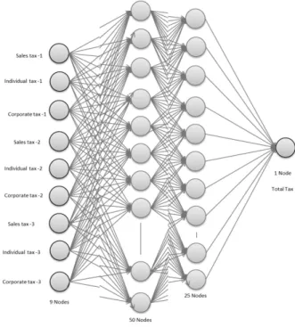
The final dataset has nine features that includes Sales Tax3, Individual Tax3, Corporate Tax3, Sales Tax2, Individual Tax2, Corporate Tax2, Sales Tax1, Individual Tax1, and Corporate Tax1. As the name implies, sales tax1, sales tax2, and sales tax3 are made from three of sales taxes. In the same way, individual tax1, individual tax2, individual tax3 are made from an individual tax. Finally, corporate tax from 1 to 3 are made from three corporate taxes. The whole number of input rows is about 513 records. As usual, several models are established and tested to find the model that shows best performance. It takes much time and effort to finish it because it must be done by manually. In this study, we have found a final model after many trials, as illustrated in Fig. 1. The model consists of four layers: one input layer, two hidden layers, and one output layer. The input layer included 9 nodes, the hidden layers included 50 and 25 nodes, and the output layer had 1 neuron. The topology is the 9- 50-25-1 topology.
Fig. 1. Topology of Artificial Neural Network Model in the Experiment
Sales Tax3
Individual Tax3
Corporate
Tax3 Sales Tax2 Individual Tax2
Corporate
Tax2 Sales Tax1 Individual Tax1
Corporate
Tax1 Total Tax
321.4 271.5 18 311.9 216.5 -3.6 319.8 372.2 175.4 670.2
311.9 216.5 -3.6 319.8 372.2 175.4 316.3 255.6 53.4 597.6
319.8 372.2 175.4 316.3 255.6 53.4 319.4 229 6.3 744.4
316.3 255.6 53.4 319.4 229 6.3 306.6 286.2 104.8 960.5
319.4 229 6.3 306.6 286.2 104.8 359.7 443 33.7 462.9
Table 2. A Sample of Extended Dataset
3.2 Implementation
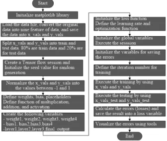
The implementation environment are as follows. The experiment system has the dual-core central processing unit (CPU) of Intel i7-3770K with 3.50 GHz and 3.90 GHz, and the memory size is 16GB. It operates over 64-bit Windows 10 operating system. The basic implementation language for implementation is Python, which has been developed by open source project. Together with this language, we have used tensor flow ANN libraries. In reality, it takes very long time to implement ANN functions when we use high-level language such as C++ or Java. Furthermore, parallel execution cannot be supported in the application. Tensorflow libraries provide all these requirements. The structure of the implementation based on Tensorflow is illustrated in Fig. 2.
To convert the original dataset into a target dataset and fit to the defined neural network model, normalize_cols function is implemented. The function split the data into train and test data by using normalization formula that use maximum and minimum value of each column. The init_weight and init_bias, are used to initialize the weight values and bias in a defined nueral network models. x_data are an array that contains input data for training. The original dataset are saved as the format of excel. These data is saved into memory, and saved in the variable. y_target contains the target data for training. Here, total tax data saved in this variable.
Fig. 2. A Flow of the Whole Implementation
The data type of both variable is two dimensional array.
The first dimension keeps the batch size, and the other contains the input and target data.
Next, fully_connected function is implemented to support fully-connected neural networks [10]. The values of each next node will be calculated by using the equation of
(weight*input_layer)+bias. The activation function used is ReLu [11]. To connect input layer with first hidden layer, weight_1 variable is defined to call init_weight function for each input node. The total number of input node is nine. The standard deviation of each input data values is 10.0. The first hidden layer includes 50 number of nodes. Here, 10.0 value of standard deviation means normal distribution with sigma standard deviation. The bias_1 variable is defined to contain the bias value of each node in hidden layers. This variable is used in the function of init_bias.
Another variable that was defined is layer_1, which is used by fully_connected function together with x_data, weight_1 variable, and bias_1 variable. By doing this, nine features is fully connected with each neuron in first hidden layer, and the results of multiplication, addition and activation function are saved in layer_1 variable.
To connect the first hidden layer with second hidden layer, along the lines of connecting input layer and first hidden layer, same kind of algorithms was implemented.
First, weight_2, bias_2 and layer_2 variable was defined and used by same functions as before. The difference is that instead of declaring input_layer in fully_connected function, layer_1 is declared, and to connect 50 hidden nodes to previous layer , the values of weight and bias inside weight_2 and bias_2 variable is set to be 50 and 10 ,respectively. In next hidden layer, 25 number of nodes are added. and multiplication with weight, addition with bias value. The results are saved in layer_2 variable.
To connect the last hidden layer to output layer, weight_3, bias_3 and final_output variable is defined. In the same way, init_weight function is called and the settings of weight inside of weight_3 is three and one. The init_bias function is also called and value of bias is 1. The reason that one more node are added is because it represent “total tax”m which will be saved in the y_target variable that only has 1 column.
Next important thing is to define a loss function[12]. The loss function is used to calculate the error in the experiment.
The result of loss function calling is saved in a separate loss variable. The loss values can be obtained by reducing the y_target by final_output and squaring the result. In our study, since we are doing batch update, all the losses of each data point in the batch need to be averaged by wrapping our normal loss function. The function is a reduce_mean() function on TensorFlow.
Next, the loss needs to be optimized. To do this, adam
optimizer is used in this study. The step values for each
iteration can be obtained by the optimization algorithm. The
distance between iteration is controlled by learning rate. The
value of the distance is 0.005. To visualize the evaluation
results, the values of training loss are saved in loss_vec array variable. In the same way, the values of testing losses test_loss variable. To optimize the algorithm, we changed the number of training and testing. For each iteration, the resulting losses are stored for every 25 intervals in a list to visualize the data and compare the results. The training and testing start by assigning to random value to x in a x_data class, and by assigning random value to y in a y_vals. The errors are stored in loss_vec array variable that has been defined earlier. The 20% of the data stored in x_data and y_target are given to the input data for testing in a defined neural network model. The losses after testing are stored in test_loss variable. To evaluate the testing results from the experiment, Matplotlib library is used for visualization [13].
The sample code of implementation is illustrated in Fig. 3.
Fig. 3. Sample Code of the Implementation
4. Results
In this section, we describes a evaluation of the implementation and experiment results from the point of training loss and testing loss. The losses are represented for each iteration in a training and testing for batch and stochastic learning using a defined neural network model.
4.1 Batch Learning
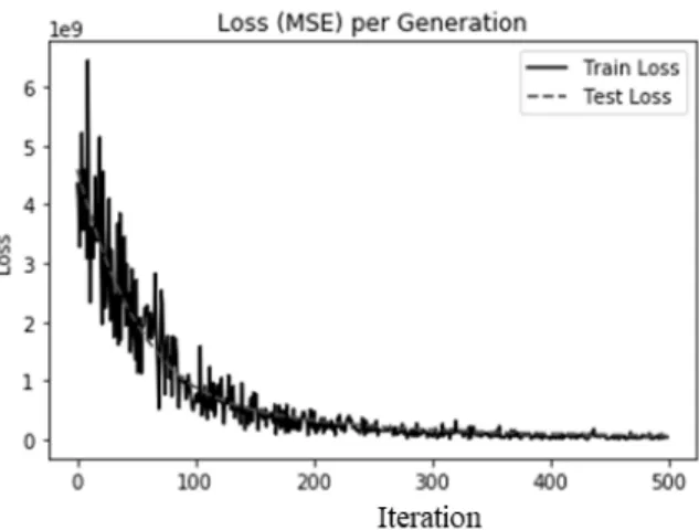
The results in a batch is illustrated on Fig. 4 and 5. Fig.
4 shows the results when batch size is set to be 10. As we can see, the loss decreases exponentially at the beginning of the iteration, and becomes stable between iteration 300 and 400. From this results, we see that only 300 iteration needs to be done until it becomes converged.
Next, we conducted an experiment with setting the batch size as 20. The results are shown in Fig. 5. As you can see from the figure, the losses start to converge between
Fig. 4. Experimental Results in a Batch with the Size of 10
Fig. 5. Experimental Results in a Batch with the Size of 20
iteration 300 and 400 too. But, the fluctuation on the training are very high when iterations are not enough. This means that a model with size of 20 is not so good when compared with the size is 10. In other words, although the errors start to decreases in same points, the result with a size of 10 is slightly better than those in twenty size of batch.
The originalities of our implementation for a batch scheme is as follows. In our scheme, we have used extended dataset that has seven features. The original dataset has three features. To enhance a performance, the dataset has been extended from original dataset. Second, we have used a TensorFlow libraries that contain efficient neural network algorithms such as parallel processing. These two schemes are different from the existing solutions.
4.2 Stochastic Learning
In this section, the experimental results are described when stochastic learning are applied. To implement the stochastic learning, the same codes with batch were used.
The different points from batch scheme are as follows.
The first is that batch size has been changed, and gradient
descent scheme is used. Therefore, the input data are given to the graph node by picking value from the input and target at random. The second is that the losses are computed, and the weights are updated by checking this loss results for every training. In a batch training, the weights are not updated according to the losses on every training. When batch is set to be 10, the weights are updated after 10 record are trained according to the resulting losses. In a stochastic, loss function has been changed into “normalization function”
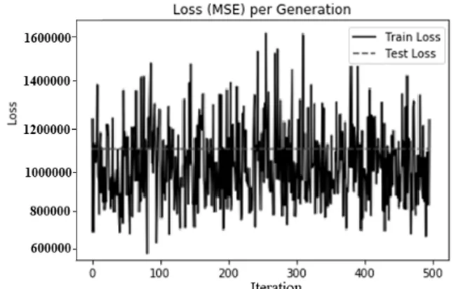
instead of “subtraction and mean“ function. The reason is that we don’t need to wrap the average of the losses. Also, batch size variable has been deleted. In a experiment for a stochastic, the iteration number was set to be the same with batch. The experimental results are represented in Fig. 6.
Fig. 6. Experimental Results in a Stochastic Model
As you can see from this figure, the performance are better than batch because the losses in the beginning of iterations are less than those in batch. The loss of the beginning in a batch was about 4.7, but, the value in a stochastic is below 1.0. This is definitely advantage. However, the fluctuation is too high from the beginning of the iteration.
This trend continues until the iteration increases, and the result does not converge stably. This is a disadvantage. A comparison between batch scheme and stochastic scheme is described in more details. From the results, we see that a batch scheme shows better performance than a stochastic model. The reason is as follows. First, starting losses at low iterations in a batch is smaller than or equal to those of a stochastic. We see that from Fig. 5, the starting loss value for training is around 2.9*10
9in a batch, and from Fig. 6, it is around 4*10
9(it is 0.4*10
10in a graph). For a staring loss for testing, both schemes have a value of 0.6 * 10
9. Second, fluctuations of losses in a batch are much lower than those in a stochastic for training and testing. This indicates that if enough training are done in a batch, the ANN can be
reliably used to predict data because it is stable. On the other hand, for a stochastic, the trained ANN cannot be used reliably although enough training has been done because there is some point where loss increases greatly.
To compare the effects for an optimizer, we have conducted an experiment by changing an original optimizer into another. In the previous experiment, we used adam optimizer. In this experiment, we used gradient descent optimizer. The code implementation to do this is very simple.
The thing to do is to simply change tf.train.AdamOptimizer to tf.train.GradientDescentOptimizer. The others were same, same code, iteration and learning rate were used. Fig.
8 represents the result for an gradient descent optimizer. As you can see from the figure, it does not converge and does not become stable. This can be used for the training. We need to analyze the causes of this results.
Next, we have conducted an experiment of learning rate changes in a stochastic with adam optimizer to improve the performance. In the previous experiment, learning rate Fig. 7. Experimental Results with Gradient Descent Optimizer
Fig. 8. Experimental Results According to the Learning
Rate Changes
distance was set to be 0.005. This value must be set in advance in optimization algorithms before each iteration. The processing time and loss minimum values are dependent on the learning rate. If the learning rate is too big, the loss might overshoot the minimum. If the learning rate is too small, it takes too much time to converge. There is no other way to find the best learning rate. We have to try to find it manually for every learning rate. In this experiment, we conducted an experiment with the rates of 0.025, 0,0025, 0.001. The experimental results are shown in Fig. 8.
As we can see from this Fig. 8-(a), if 0.025 learning rate is set be 0.025, the loss overshoot the minimum. With 0.0025 learning rate, it start to converge between 400 and 500 iteration as shown in Fig. 8-(b). With 0.001, it dose not converge until 500 iterations as shown in Fig. 8-(c). In this case, it need more iteration to converge.
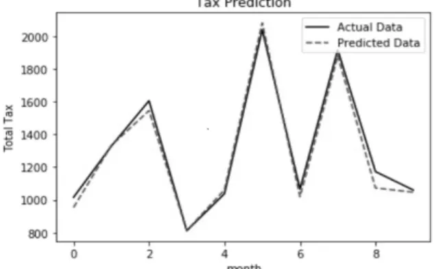
4.3 Prediction Results
In this section, prediction results of taxes are described.
We collected real data about taxes from official website in Indiana State in USA, and predicted the taxes using trained neural networks. Then, we compared each data. In this experiment, we have used a neural network model with a 9-50-25-1 topology to predict the total taxes. Also, a stochastic model [14] was used to train the model. It takes from twenty to thirty minutes to train the model to achieve the convergence. Table 3 shows the results of the measurement and prediction.
Date Actual Total Tax Predicted Total Tax
February 2018 965.3 965.4917
March 2018 1907 1907.5023
April 2018 1405.8586 1406.1
May 2018 1,136.7 1094.3425
June 2018 1123.8 1046.3466
July 2018 1116.1 1185.5496
August 2018 1000.9 1070.29406
September Not published yet 1537.664 Table 3. A Comparison of Predicted and Actual Taxes
After september, the available data was not released.
From the collected data, we take the total tax on the last field in the dataset. From this result, we see that the predicted results are almost same with the real data. The accuracy result is really good. A model of a neural networks is defined as the number of layers and the number of neurons for each layer. As usual, one more models are defined, trained, and tested by developers using input dataset. Then, the best model is chosen after evaluating each
model. In our experiment, it is determined that a 9-50-25-1 topology is the best model. The experiment results reveals that the trend of predicted taxes is almost similar to that of actual taxes. Fig. 9 shows a comparison of actual and predicted total taxes.
Fig. 9. A Comparison of Actual Tax and Predicted Taxes
5. Conclusion
In this study, a batch based ANN model and stochastic ANN model have been implemented using TensorFlow libraries. Each model are evaluated by comparing training and testing errors that are measured through experiment. To train and test each model, tax dataset was used that are collected from the government website of indiana state budget agency in USA from 2001 to 2018. The dataset includes tax incomes of individual, product sales, company, and total tax incomes.
The experimental results show that batch model reveals better performance than stochastic model. Using the batch scheme, we conducted an experiment in which total taxes are predicted during next seven months, and compared with actual collected total taxes. the results shows that predicted data are almost same with the actual data.
The future works is to improve the processing time and decrease the losses. To reduce the processing time, parallel processing can be used. In a parallel processing scheme, input dataset for training and testing are divided into smaller parts, and each data are stored in distributed clients computing devices. Then, the results are merged into one final data.
References
[1] L. Sheng, C. Zhong-jian, and Z. Xiao-bin, “Application of
GA-SVM time series prediction in tax forecasting,” 2009 2nd
IEEE International Conference on Computer Science and
Information Technology, Beijing, 2009, pp.34-36.
[2] Y. Zhang, “Research on the Model of Tax Revenue Forecast of Jilin Province Based on Gray Correlation Analysis,” 2014 Sixth International Conference on Intelligent Human-Machine Systems and Cybernetics, Hangzhou, 2014, pp.30-33.
[3] D. Liu, R. Zhang, and J. Li, “Tax Revenue Combination Forecast of Hebei Province Based on the IOWA Operator,”
2011 Fourth International Joint Conference on Computational Sciences and Optimization, Yunnan, 2011, pp.516-519.
[4] D. Sena and N. K. Nagwani, “Application of time series based prediction model to forecast per capita disposable income,”
2015 IEEE International Advance Computing Conference (IACC), Banglore, 2015, pp.454-457.
[5] T. W. Ayele and R. Mehta, “Real Time Temperature Prediction Using IoT,” 2018 Second International Conference on Inventive Communication and Computational Technologies (ICICCT), Coimbatore, 2018, pp.1114-1117.
[6] T. W. Ayele and R. Mehta, “Air pollution monitoring and prediction using IoT,” 2018 Second International Conference on Inventive Communication and Computational Technologies (ICICCT), Coimbatore, 2018, pp.1123-1132.
[7] Y. Wang, J. Zhou, K. Chen, Y. Wang, and L. Liu, “Water quality prediction method based on LSTM neural network,”
2017 12th International Conference on Intelligent Systems and Knowledge Engineering (ISKE), Nanjing, 2017, pp.1-5.
[8] A. M. Ertugrul and P. Karagoz, “Movie Genre Classification from Plot Summaries Using Bidirectional LSTM,” 2018 IEEE 12th International Conference on Semantic Computing (ICSC), Laguna Hills, CA, 2018, pp.248-251.
[09] K. Greff, R. K. Srivastava, J. Koutník, B. R. Steunebrink, and J. Schmidhuber, “LSTM: A Search Space Odyssey,” in IEEE Transactions on Neural Networks and Learning Systems, Vol.28, No.10, pp.2222-2232, Oct. 2017.
[10] G. Botla, V.K. Vadlagattu, and Y. R. Kalipatnapu, “Modeling of Batch Processes Using Explicitly Time-Dependent Artificial Neural Networks,” in IEEE Transactions on Neural Networks and Learning Systems, Vol.25, No.5, pp.970-979, 2014.
[11] Y. A. Alma, “Electricity Prices Forecasting using Artificial Neural Networks,” in IEEE Latin America Transactions, Vol.16, No.1, pp.105-111, 2018.
[12] R. Saman, and A. T. Bryan, “A New Formulation for Feedforward Neural Networks,” in IEEE Transactions on Neural Networks, Vol.22, No.10, pp.1588-1598, Oct. 2011.
[13] W.-C. Yeh, “New Parameter-Free Simplified Swarm Optimization for Artificial Neural Network Training and its Application in the Prediction of Time Series,” in IEEE Transactions on Neural Networks and Learning Systems, Vol.24, No.4, pp.661-665, 2013.
[14] Y. Weizhong, “Toward Automatic Time-Series Forecasting Using Neural Networks,” in IEEE Transactions on Neural Networks and Learning Systems, Vol.23, No.7, pp.1028-1039, 2012.
Kumbayoni Lalu Muh
https://orcid.org/0000-0002-2342-4645
e-mail : [email protected] He received a bachelor from degree in Automotive Engineering from Daegu Catholic University in 2017. He is workng on MSd in Kumoh National Institute of Technology. His research interests are in the area of Machine Leaning, Image recognition, Artificial Neural Network.
Sung-Bong Jang
https://orcid.org/0000-0003-3187-6585