A Study on Simultaneous Adjustment of GNSS Baseline Vectors and Terrestrial Measurements
Nguyen, Dinh Huy1)·Lee, Hungkyu2)·Yun, Seonghyeon3) Abstract
GNSS (Global Navigation Satellite System) is mostly used for high-precise surveys due to its accuracy and efficiency. But this technique does not always fulfill the demanding accuracy in harsh operational environments such as urban canyon and forest. One of the remedies for overcoming this barrier is to compose a heterogeneous surveying network by adopting terrestrial measurements (i.e., distances and angles). Hence, this study dealt with the adjustment of heterogeneous surveying networks consisted of GNSS baseline vectors, distances, horizontal and vertical angles with a view to enhancing their accuracy and so as to derive an appropriate scheme of the measurement combination. Reviewing some technical issues of the network adjustments, the simulation, and experimental studies have been carried out, showing that the inclusion of the terrestrial measurements in the GNSS standalone overall increased the accuracy of the adjusted coordinates. Especially, if the distances, the horizontal angles, or both of them were simultaneously adjusted with GNSS baselines, the accuracy of the GNSS horizontal component was improved. Comparing the inclusion of the horizontal angles with those of the distances, the former has been more influential on accuracy than the latter even though the same number of measurements were employed in the network.
On the other hand, results of the GNSS network adjustment together with the vertical angles demonstrated the enhancement of the vertical accuracy. As conclusion, this paper proposes a simultaneous adjustment of GNSS baselines and the terrestrial measurements for an effective scheme that overcomes the limitation of GNSS control surveys.
Keywords : Global Navigation Satellite System, Terrestrial Measurements, Heterogeneous Network, Network Adjustment, Accuracy
1. Introduction
High precision of GNSS positioning techniques has become an essential tool for surveying and mapping applications by delivering unprecedented accuracy and efficiency. As well known, GNSS surveying with the carrier-phases on stationary mode efficiently delivers a few centimeters level of positioning accuracy in the horizontal and the vertical component; hence, it has been mainly used for the control and the deformation surveys. Nevertheless,
GNSS has the inherent drawback which requires line-of-sight between a receiver antenna and satellites; hence positioning is difficult and even impossible at a site where satellite signals are insufficient, such as an urban canyon and a valley in a mountain. Additional shortcomings can be low accuracy in the vertical component due to the geometry of the satellite constellation.
For kinematic positioning and navigation applications, appropriate integration of GNSS with INS (Inertial Navigation System) or IMU (Inertial Measurement Unit)
Received 2020. 09. 12, Revised 2020. 10. 07, Accepted 2020. 10. 21
1) Member, Dept. of Geodesy and Geomatic, Lecturer, National University of Civil Engineering (NUCE), Vietnam (E-mail: [email protected]) 2) Corresponding Author, Member, School of Civil, Environmental and Chemical Engineering, Professor, Changwon National University (E-mail:
3) Member, Dept. of Eco-Friendly Offshore Plant FEED Engineering, Ph.D. student, Changwon National University (E-mail: [email protected])
https://doi.org/10.7848/ksgpc.2020.38.5.415 Original article
This is an Open Access article distributed under the terms of the Creative Commons Attribution Non-Commercial License (http://
creativecommons.org/licenses/by-nc/3.0) which permits unrestricted non-commercial use, distribution, and reproduction in any
can effectively address the intrinsic limitation of the GNSS technology (Farrel and Barth, 1999; Grewal et al., 2001). On the other hand, a simultaneous adjustment of GNSS and some terrestrial surveying measurements obtained by a TS(Total Station), such as distances and angles, can remedy the drawback of the standalone GNSS positioning for static applications, for instance, geodetic and cadastral control surveys and deformation monitoring of civil engineering structures and landslides (Valev and Minchev, 1995; USACE, 2002; Ilie, 2016). Although such technology especially has high applicability in Korea due to urbanization and mountainous terrain, a literature review has discovered only a few research activities dealt with the GNSS and terrestrial measurements. Shin et al. (2000) carried out experimental research of joint observations by GNSS and TS for the cadastral surveys in the downtown area where the satellite signal blockage occurred frequently.
Lee et al. (2000) analyzed geodetic characteristics of the old- triangulation surveys of the Guam local system by GNSS and TS campaign. Kim (2001) proposed a combined approach of GNSS with TS for monitoring an earth dam. Nonetheless, the researches mentioned above did not attempt to combine the heterogeneous measurements by the least-squares, known as the most rigorous estimation technique in geodesy. Although Lee et al. (2008) simultaneously processed GNSS baseline vectors and EDM (Electromagnetic Distance Measurement Unit) distances, it only focused on deriving an adjusting procedure of GNSS and distance observations for densification of the KGD2002 (Korean Geodetic Datum 2002).
In this contribution, heterogeneous networks comprised of GNSS-estimated baseline vectors and TS-measured angles and distances have comprehensively been processed and analyzed to demonstrate the potential benefits of such an approach in terms of accuracy and to derive an appropriate scheme of the surveying data combination. The remainder of this paper is as follows. Some technical issues related to the adjustment of the heterogeneous network are firstly addressed with an emphasis on the importance of stochastic modeling. This is followed by describing details of simulation and experimental analysis on the network adjustments via various combinations of GNSS and terrestrial measurements.
Finally, the research findings and conclusions are summarized, and recommendations for future studies are made.
2. Technical Issues of the Heterogeneous Network Adjustment
The geodetic and surveying network is a mathematical process that estimates coordinates of unknown points from a set of measurements. The least-squares principle is generally applied to distributing random errors of the observations throughout the network; hence, the adjusted measurements conform to geometric conditions or other required constraints. In addition to the coordinate estimation during the adjustment, a series of statistical tests are performed not only to examine the fidelity of a mathematical model but also to identify and adapt outliers; and a geodetic datum of the network is defined. Therefore, the adjustment results in coordinates together with their absolute accuracy and relative accuracy of the network. Note that the accuracy is commonly represented by an error ellipse and/or an error bar with a specified confidence interval.
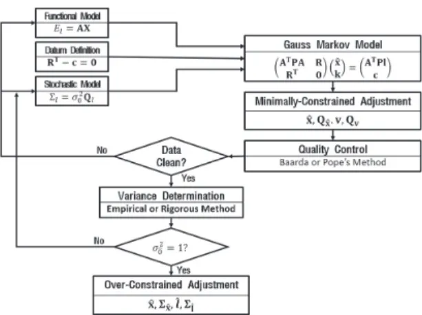
As shown in Fig. 1, an optimal mathematical model should be established for the network adjustment. The GMM (Gauss- Markov Model) is a model consisting of functional and stochastic relations. While the functional model describes the mathematical relationship between observations and unknown parameters to be estimated, the stochastic model represents precision and correlation of measurements.
Although the functional models can be formulated either on a reference surface or in a 3-dimensional (hereafter 3D) space, the latter approach is more straightforward to the heterogeneous network considered in this study as GNSS- estimated baseline vectors are included, and terrestrial measurements, such as angles and distances, do not need to be reduced to the reference surface. The 3D models for the traditional surveying measurements were well documented, e.g., see Thomas (1976) and Steeves (1994). On the other hand, stochastic modeling for an inhomogeneous network has technical challenges as the precision of each measurement is unknown. In order to rigorously model it, the variance component estimation techniques can be used, but they usually need much computational burden (Caspary, 2000).
To this end, an empirical modeling scheme, which is simple and effective, has practically been employed in this study. In this technique, each type of measurement set is separately
and iteratively adjusted by applying an initial variance until all possible outliers are isolated, and a posterior variance of the last repetition is finally determined as a scale factor for refinement of a provisional cofactor matrix.
Fig. 1. A general procedure of the surveying network adjustment
Two classes of network adjustments are separately conducted: (a) ‘the MCA (Minimally Constrained Adjustment)’; (b) ‘the over or FCA (Fully Constrained Adjustment).’ The minimum number of the known points required for defining a datum is held fixed in the MCA to avoid rank deficiency of a design matrix (A) and to exempt errors of control stations. The primary roles of the MCA are to identify and adapt possible outliers by the Baarda or Pope’s method and to assess the internal consistency of a network, which can be represented by a relative error ellipse and bar.
For a heterogeneous adjustment in this research, the MCA for each type of measurements (e.g., baseline vectors, angles, and distances) was independently performed for quality control and determination of a reference variance. And then, that of the combined network was carried out to verify the existence of outliers further and to define a reference variance again.
Of course, the results of the second round should confirm the unity of a posterior variance. As a final step of the adjustment, the fully or OCA (over constrained adjustment) is conducted by constraining all available control stations in the network, estimating coordinates of unknown points with quality measures, such as a posterior variance and a cofactor matrix of unknown parameters(e.g., and ).
3. Simulation Analysis
3.1 Network design
The surveying network simulation is a technique that overall evaluates and verifies the accuracy and reliability of a network through propagating observations errors. Actual measurements are not required in this process, which is a benefit of this technique, but network configuration and magnitude errors should be defined by a design matrix (A) and a variance-covariance matrix for observables( ). As shown in Fig. 2, a simulation network was composed of 29 points. To define the design matrix, the published coordinates of the three national geodetic control points, i.e., TR360, TR24, and CHWN, were adopted, and those of the unknown points were extracted from the Google Map.
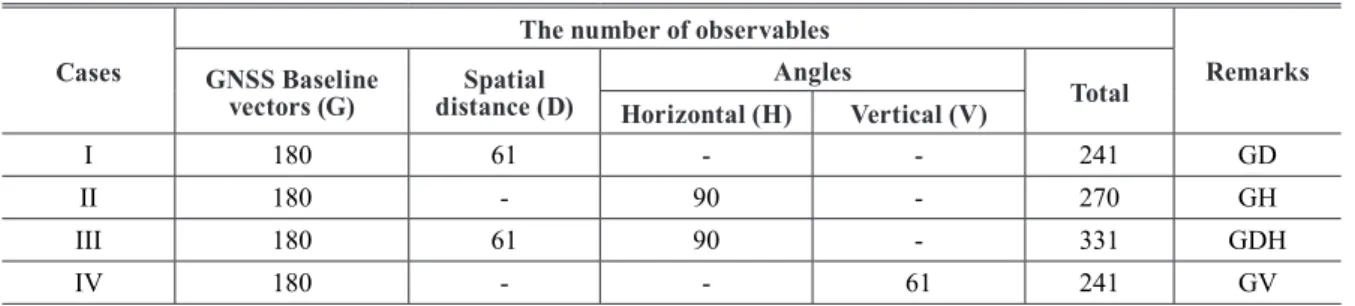
Fig. 2. Network configuration for simulation analysis As given in Table 1, four testing cases, depending on a combination of measurement types, were arranged for the simulation to analyze the influence of the terrestrial observations into a GNSS network. Note that the surveying measurements considered in the analysis are GNSS-estimated 3D baseline vectors, spatial distances, and horizontal and vertical angles. In the functional modeling, several assumptions were made for the observable acquisition, such as three GNSS receivers, distance and vertical angles between the points, and inner horizontal angles of the triangles in the network diagram. To this end, the number of GNSS baseline vectors, distances, horizontal angles, and vertical angles are 60, 61, 90, and 61, respectively, as shown
in Table 1. Additionally, Table 1 tabulates the number of observations of each testing cases included in the simulation cases. On the other hand, for stochastic modeling, only variance values were defined without correlations to each type of the observables as:
(a) the site and baseline dependent constants were defined for the GNSS baseline vectors and distances, for instance, 4mm+0.5PPM and 8mm+1PPM for the horizontal and the vertical component of the GNSS baseline vectors, and 2mm+2PPM for the distances;
(b) the reading and pointing error represented by the DIN- 18723 standard (e.g., ±3“) together with the 2mm of the mis-centering are considered in the angle observables.
3.2 Processing and results
The processing began with MCA and OCA of the homogeneous networks to verify their mathematical models and obtain a reference accuracy for the following analysis, especially the GNSS network. This was followed by conducting OCA of the heterogeneous networks (i.e., cases I to IV). However, it is of importance to take note that only horizontal coordinates are set as unknown parameters in the functional model of the distances due to the limitation of the software used in this study. Since the three control stations in Fig. 2 were held fixed in the processing, the number of unknown parameters was 78 for all the cases, but the DoF (Degree of Freedom) varied with the cases. As an example, a network diagram of the case IV, together with absolute error ellipses and bars with 95% of the confidence interval is given in Fig. 3.
Cases
The number of observables
Remarks GNSS Baseline
vectors (G) Spatial
distance (D) Angles
Total Horizontal (H) Vertical (V)
I 180 61 - - 241 GD
II 180 - 90 - 270 GH
III 180 61 90 - 331 GDH
IV 180 - - 61 241 GV
Table 1. Testing cases and configuration of observables
Fig. 3. A processed network of the case IV with error ellipses and bars at a 95% probability
While Table 2 summarizes sizes of the semi-major axes of the absolute error ellipse and the lengths of the error bar with a 95% probability, characterizing the confidence interval (i.e., accuracy) of the estimation coordinates in the network simulation, Fig. 4 depicts averages and standard deviations of the sizes. It is worth observing the changes of the values in the results rather than the absolute values themselves as they vary with the stochastic models defined to each an observable set. Therefore, the level of the accuracy enhancement in the seven cases, compared to the GNSS only, is tabulated in Table 2, which demonstrates the impact of the terrestrial measurements on the GNSS network. As intuitively expected from the composition of the measurement types in the cases, the horizontal angels and the distances mostly contribute to the horizontal component, whereas the vertical angles influence that of the vertical.
More importantly, a focus should be given on the level of the accuracy improvement, for instance, 19.7% and 27.6%
in the horizontal estimation on average by including the distances and the horizontal angles, and 40.9% in the height estimation by the vertical angles. Notably, it is interesting to see that comparing the horizontal angles with the distances, the impact of the former has more impact on the accuracy even though the same number of measurements are included in the processing. If both the traditional measurements are adjusted with the GNSS baseline vectors, the accuracy is improved by 34.2% on average. To this end, if the GNSS surveys do not fulfill the accuracy specification for some applications, especially deformation surveys, the simulation results give a clue in which the combination of GNSS and terrestrial measurements overcomes the limitation. For such an application, the simulation analysis can play an essential role in the design stage.
Fig. 4. Averages and standard derivations of size of the error ellipses and bars at a 95% confidence level (unit: mm)
Table 2. Summary of the absolute accuracy of testing cases at a 95% confidence level CASES
Semi-major Axis Error bars
Remarks Average
(mm) Improve-
ment(%) Std. Dev.
(mm) Max.
(mm) Average
(mm) Improve-
ment(%) Std. Dev.
(mm) Max.
(mm)
G 7.6 - ±1.2 9.4 18.1 - ±2.1 22.4 GNSS only
GD 6.1 19.7 ±1.0 6.9 18.1 0.0 ±2.1 22.4 GNSS & Distance
GH 5.5 27.6 ±1.0 6.4 18.1 0.0 ±2.1 22.4 GNSS &
Horizontal angle GDH 5.0 34.2 ±1.0 6.0 18.1 0.0 ±2.1 22.4 GNSS, Distance & Horizontal angle
GV 7.6 0.0 ±1.2 9.4 10.7 40.9 ±1.2 13.3 GNSS & Vertical
angle
4. Experiment and Analysis
4.1 Field surveys
A field surveying campaign was carried out to verify the results of the simulation studies that focused on investigating the effect of the inclusion of terrestrial measurements on GNSS network adjustment. Fig. 5 depicts an experimental network on the campus of the Changwon National University, South Korea. A total of eight surveying points was included in the network, composing of two control stations (i.e., CHWN, U0982) and six unknown points in order from T01 to T06.
Three geodetic-grade receivers (e.g., Javad Alpha, Sokkia GRX1) were used for the field campaign to obtain GNSS observations on static mode. Dual-frequency measurements were observed with 5 seconds sampling rate for an hour at each point. The adjacent sessions were connected by two common stations, and a total of 6 sessions was obtained as presented in Fig. 5. The antenna height was measured twice to the millimeter; after that, rinex-formatted GNSS observations were processed by LGO (Leica Geo Office) to estimate 3D baseline vectors between the points. Note that only independent baselines were dealt with this processing;
hence, a total of 39 baseline vector components and their VCV (Variance-Covariance) matrix were obtained for the following adjustments. A TS, Topcon GTS-723, was used to acquire terrestrial measurements. The distances and vertical angles between the points, and inner horizontal angles of the triangles in the experimental network were measured; thus, terrestrial measurements consisted of 15 slope distances, 15 horizontal angles, and 12 vertical angles. On the other
hand, for stochastic modeling, the standard deviation of these measurements was determined based on the equipment specification. That was, 2mm+2PPM for the distances and ± 3" (DIN 18723) for the angles together with the mis-centering errors (e.g., 2mm).
Fig. 5. A layout of the experimental network
4.2 Adjustments and results
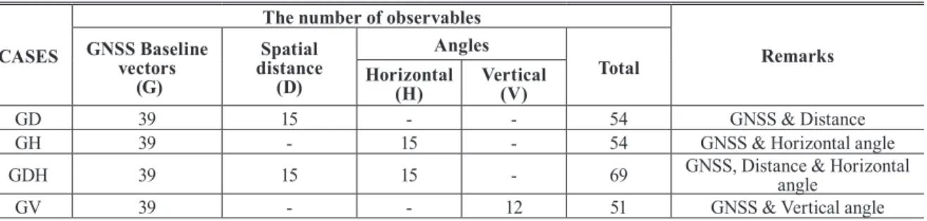
To examine the effect of terrestrial measurements on an adjustment of the GNSS network, four cases, as summarized in Table 3, were designed for types of observations included.
Note that the number of distances and horizontal angles is identical, ensuring that they similarly contributed to an increasing number of observations in the networks.
MCA of the homogeneous networks (e.g., GNSS, distances, angles) have been independently performed to examine outliers and also to refine initial stochastic models.
Table 3. Testing cases and their observations in the experimental cases CASES
The number of observables
Remarks GNSS Baseline
vectors (G)
Spatial distance
(D)
Angles
Total Horizontal
(H) Vertical
GD 39 15 - (V)- 54 GNSS & Distance
GH 39 - 15 - 54 GNSS & Horizontal angle
GDH 39 15 15 - 69 GNSS, Distance & Horizontal
angle
GV 39 - - 12 51 GNSS & Vertical angle
From the adjustment, no blunder was fortunately identified and posterior scaling factors for TS observations were determined. On the other hand, the stochastic model of the GNSS baselines was refined by the so-called empirical modeling technique (Rizos, 1997), resulting in 4mm+0.8 PPM for the horizontal and 8mm+1PPM for the vertical components.
MCAs of the seven heterogeneous networks have been conducted in turn to further confirm the existence of outliers and the stochastic models. Throughout this process, the unity of a posteriori variance value was statistically verified by Chi-square tests. After that, the OCA of the combined networks were successively processed by constraining the known stations, so as to estimate the final coordinate sets with their accuracy represented by error ellipses and bars. As an example, a network diagram of the case GDHV, together with absolute error ellipses and bars at 95% of the confidence level is given in Fig. 6.
Fig. 6. A processed network of the GV case with error ellipses and bars at a 95% probability
While Table 4 statistically summarizes the absolute accuracies of the estimate coordinates, Fig. 7 presents the averages and the standard deviation of the accuracy measures.
Comparing the accuracy of the heterogeneous network with that of the standalone GNSS, the formers are generally more accurate than that of the latter. However, the level of the accuracy enhancement depends upon the observational composition, as seen in Table 4. For instance, the horizontal accuracy is increased by 12.9% and 14.9%, with the inclusion of the distances and horizontal angles. On the other hand, the vertical estimation of the combined network becomes 22.1% accurate by the contribution of the vertical angles.
Table 4 also demonstrates that the maximum error of both horizontal and vertical components is significantly decreased by adding terrestrial measurements to the GNSS network.
For instance, the largest size of the error bars in GV is almost two times smaller than the G case. Even though the number of the distances and the horizontal angles are identical in the heterogeneous composition, it can be seen from the results that the latter is more influential on accuracy than the former.
To the end, the addition of the traditional measurements with the GNSS baseline vectors is an effective way not only to improve the accuracy of the GNSS network but also to substitute the GNSS network in where satellite signals are insufficient.
Table 4. Summary of the absolute accuracy of testing cases at a 95% confidence level
Fig. 7. Absolute accuracy of the adjustments at a 95%
confidence level, including their means and standard deviations (unit: mm)
Coordinate differences between the GNSS standalone and the combination were driven to study the reality of the contribution of the terrestrial contribution on a GNSS network.
The averages and standard deviations of the differences in the horizontal and vertical components are summarized in Table 5 and further depicted in Fig. 8. As shown in Table 5, the averages of the horizontal are 1.3mm, 1.5mm, and 1.6mm for the GD, GH, and GDH cases, respectively. The value of the GV horizontal component is relatively small (i.e., 0.2mm), while that of the vertical direction is 1.4mm. Such a result can be considered to be reasonable as the vertical accuracy of the GNSS network is only significantly improved by adding the vertical angles.
CASES Semi-major Axis Error bars
Average
(mm) Improve-
ment (%) Std. Dev.
(mm) Max.
(mm) Average
(mm) Improve-
ment (%) Std. Dev.
(mm) Max.
(mm)
(GNSS only)G 10.1 - ±3.6 14.4 19.9 - ±7.0 28.0
(GNSS & Distance)GD 8.8 12.9 ±2.6 10.6 19.8 0.5 ±6.8 27.3
(GNSS & Horizontal)GH 8.6 14.9 ±2.4 10.2 19.8 0.5 ±6.7 27.0
(GNSS, Distance & GDH
Horizontal angle) 8.2 18.8 ±2.3 9.7 19.9 0.0 ±6.5 26.4
(GNSS & Vertical angle)GV 9.3 7.9 ±3.2 12.7 15.5 22.1 ±4.2 14.7
Fig. 8. Adjusted coordinates difference and their standard deviations (unit: mm)
5. Concluding Remarks
In this paper, the scheme of the surveying data combination has been reviewed with an emphasis on the importance of stochastic modeling, so as to demonstrate the potential benefits of such an approach in terms of accuracy as well as to derive an optimal way to adjust a heterogeneous geodetic network. A series of simulation and experimental analyses have been intensively carried out to assess the level of accuracy enhancement of the heterogeneous network with the GNSS network standalone. Particularly, the horizontal accuracy of the GNSS network is increased by 12.9%, 14.9%, and 18.8% with the inclusion of spatial distance, horizontal angles, and both of them, respectively. On the other hand, the horizontal angle has more impact on the accuracy than the distance, even though the same number of measurements are included in the processing. The accuracy of vertical direction
Table 5. Statistics of the difference coordinates between testing cases and GNSS network
CASES Horizontal component Vertical component Remarks
Aver. (mm) Std. (mm) Aver. (mm) Std. (mm)
GD 1.3 1.4 0.6 0.4 GNSS & Distance
GH 1.5 1.3 0.7 0.6 GNSS & Horizontal angle
GDH 1.6 1.4 0.9 0.6 GNSS, Distance & Horizontal angle
GV 0.2 0.2 1.4 1.7 GNSS & Vertical angle
is improved by 22.1% when the GNSS baseline vector is simultaneously adjusted with the vertical angles. Hence, the addition of the vertical angles in the GNSS network is an effective way to enhance its vertical accuracy. However, it should be noted that the conclusion was derived from the analysis of specific experiments in this study; hence, these results would be somewhat diverse if different conditions are applied in the adjustments. Nevertheless, on some sites where GNSS signals are blocked in an urban canyon, and forest or surveying accuracy does not fulfill its tolerance, the simultaneous adjustment of the heterogeneous network is proposed for an alternative method estimating the high accuracy of 3-D coordinate sets.
Acknowledgment
This research has been partially supported by the National Research Foundation of Korea (NRF-2014R1A1A2056133).
References
Caspary, W.F. (2000), Concepts of Network and Deformation Analysis, Monograph No. 11, School of Geomatic Engineering, University of New South Wales, Australia, 185p.
Farrell, J.A. and Barth, M. (1999), The Global Positioning System and Inertial Navigation, McGraw-Hill Companies, Inc., New York.
Grewal, M.S., Weill, L.R., and Adnrews (2001), Global positioning systems, inertial navigation, and integration, John Wiley & Sons, Inc., New York.
Ilie, A.S. (2016), Adjusting 3D geodetic network using both global navigation satellite systems technology (GNSS) and
terrestrial measurements, Environmental Engineering and Management Journal, Vol. 15, No. 6, pp. 1223-1235.
Kim, J.S. (2001), A study on the Deformation Monitoring for Earth Dam by GPS and TS, Doctoral dissertation, Dong-A University, Busan, Korea, 154p.
Lee, Y.J. and Kim, H.I. (2000), Analyses of the old- triangulation survey of the Guam-System by GPS/TS, Journal of the Korean Society of Cadaster, Vol. 16, No. 1, pp. 55-68. (in Korean with English abstract)
Lee, Y.J., Lee, H.K., Jeong, K.H., and Song, J.H. (2008), Integrated adjustment test of GPS/EDM observations for accuracy improvement, Journal of the Korean Society of Cadaster, Vol. 24, No. 1, pp. 245-255. (in Korean with English abstract)
Rizos, C. (1997), Principle and Practice of GPS Surveying, School of Surveying and Spatial Information Systems, The University of New South Wales, Sydney, Australia.
Shin, S.C., Seo, C.S., and Kim, J.D. (2000), Some solutions of the GPS/TS positioning in cadastral surveying, Journal of the Korean Society of Cadaster, Vol. 1, No. 1, pp. 69-81.
(in Korean with English abstract)
Steeves, R. R. (1984), Mathematical Models for Use in the Readjustment of the North American Geodetic Networks, Technical Report No. 1, Geodetic Survey of Canada, Canada.
Thomson, D.G. (1976), Combination of Geodetic Networks, Technical Report No. 30, Department of Surveying Engineering, University of New Brunswick, Canada.
USACE (2002), Engineering and Design: Structural Deformation Surveying, Engineering Manual, US Army Corps of Engineers, Washington, DC, 302p.
Valev, G. and Minchev, M. (1995), Combined adjustment of GPS and classical network data, Report Symposium of the IAG Subcommission for EUREF, 3-6 May, Helsinki, Finland, pp. 213-220.